Weekly solutions, tidal analysis of the Onsala SCG, GWR #54

GGP station OS

Most recent solution is from observations 2009-JUN-15 to 2024-APR-11
Check for errors

This page was revised 2022-01-24

Select:

1. Diagrams of residual and a few time series (drift model and atmospheric and Kattegatt sea level effects).
   Note that the extended analysis uses a tighter outlier criterion.
2. Power spectrum of the "raw" residual and of the noise-whitened residual ( log-f raw, log-f whitened)
   
from the Standard analysis.
3. Result sheets:  Standard analysis   | Simple (with local air pressure) (delta-factors and admittance coefficients)
4. Gain and Phase spectrum of gravity effect due to Kattegat
   
5. Diagram of the atmospheric components scaled by the estimated admittances from the standard analysis.
   

Result sheet - glossary

Standard analysis: Signal model comprises

• SG series decimated to 1 Sph
• Predicted gravity from polar motion
  
• Atmacs Newtonian part, local, regional and global added together, long-period tides removed, Wiener filtered to preserve periods greater than 1 cyc/day
• Local barometer, Wiener filtered to preserve periods less than 1 cyc/day as a complement to the above
  
• Local barometer, Wiener filtered to adapt to SG residual (remainder effects)
  
• Atmacs global loading
• Local tide gauge, barometer added as a proxy for bottom pressure
• Nodal tide, subtracted from SG (no coefficient solved for)
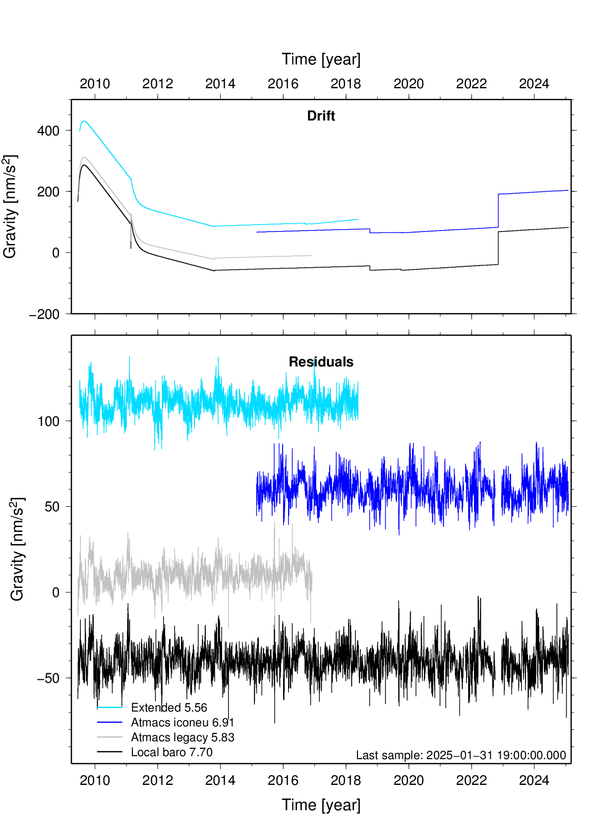
• Drift model
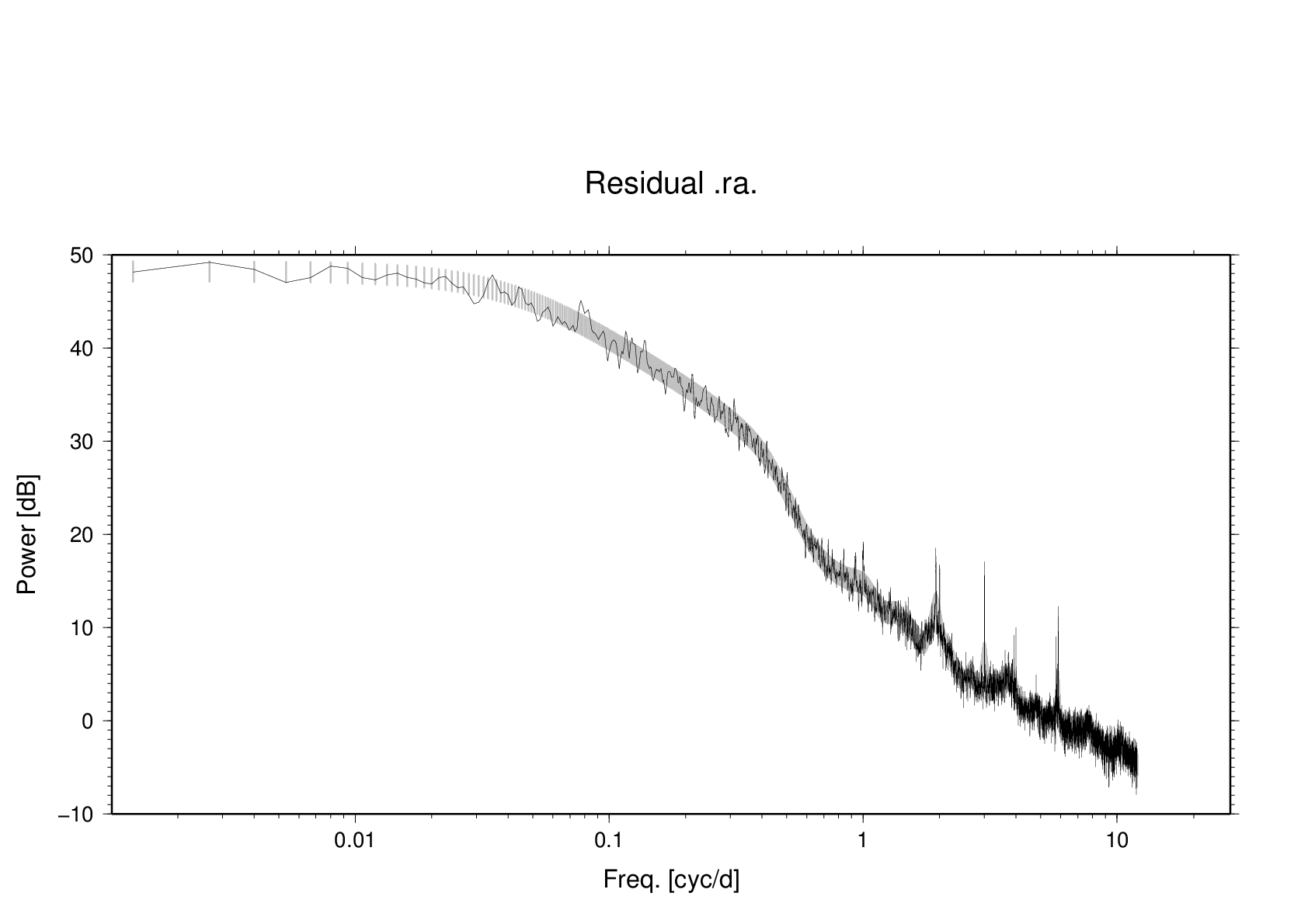
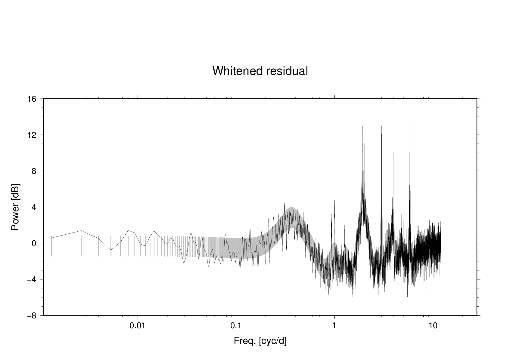
• All series are filtered with a Prediction-error filter (PEF) in order to whiten the residual noise.
  

Extended analysis, will be exercised only causally. Signal model comprises standard setup plus

• Ecco1 non-tidal ocean model, predicted gravity, from loading.u-strasbg.fr
• ERAin hydrosphere, predicted gravity, from loading.u-strasbg.fr
  

DELTA SYSTEM: DEHANT - Delta factors are ratios of the observable earth tides with respect to the predicted effect on a rigid earth.

Tide symbols: The Tamura (1987) potential is used. Table 1 at the end shows the wavegroup selection.

3-0, 3-1, 3-2, and 40-1: Degree-n order-m tides where 3 ≤ n ≤ m are treated separately from the leading terms (n = 2, 0 ≤ m ≤ 2); however, the degree-4 tides have been put into one signal band (0 ≤ n ≤ 3, m = 4).  

Atmacs - an atmospheric prediction model of gravity perturbations, provided by BKG, Germany.

RIOS - Combined tide gauges at Ringhals (until 2013-08-27) and Onsala (thereafter), coast of Kattegat. Ringhals, located 18.5 km SE of Onsala, is equipped with a stilling gauge, resolution 1 cm, 1 hour. Since summer 2013 a "bubbler" gauge has been in operation at Onsala (resolution 0.1 mm, 1 min). The air pressure at Onsala has been added to obtain a proxy for loading-effective sea bottom pressure.
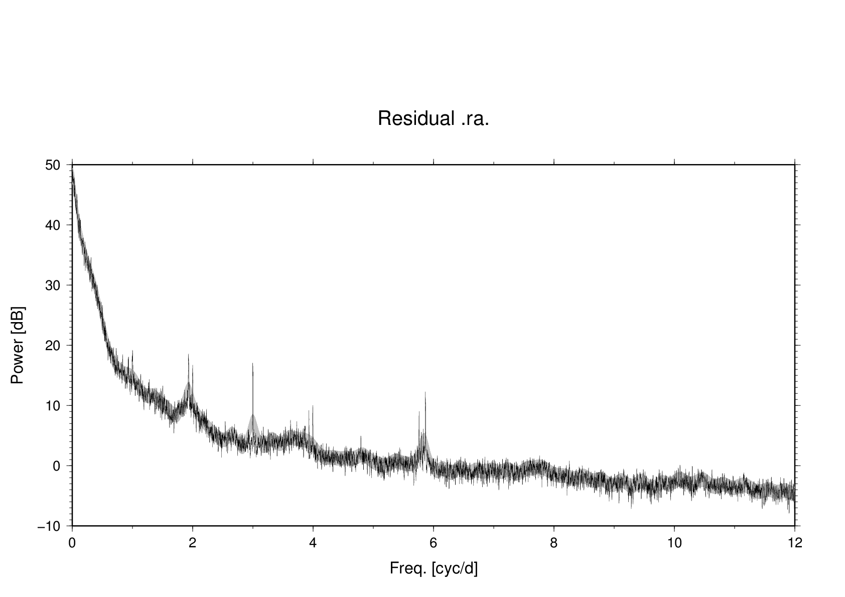
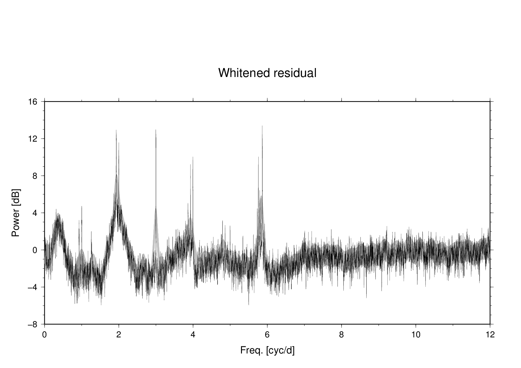
     In the weekly-extended gravity solutions the ocean tide has been reduced from this time series (which includes four waves in the M₆ band, nota bene). Nevertheless, the power spectrum exhibits residual tidal signal power, prominently at semi-diurnal periods; The M₆ (1/6 of the lunar day) in the gravimeter record is not solved at all, so the residual contains its full power. The M₂ residual, however, prompts for an explanation.
      In the least-squares tide solution a stationary average tide is removed; the remainder is a non-stationary component, which is picked up by the power spectrum, since it is not based on the long-term behaviour. but rather on the autocovariance within a 4092 hours Kaiser-Bessel (parameter 2.2) window.
     The loading-effective bottom pressure is associated with a mass imbalance. We would need to run a realistic ocean tide model with pressure and wind included in the forcing in order to resolve what an area the imbalance is confined to, probably a momentary property changing with the weather patterns. On average, 1 hPa of bottom pressure increase as measured at the beach (10 kg per square meter, 1 cm water head) causes gravity  to increase with 0.13 to 0.14 nm/s².

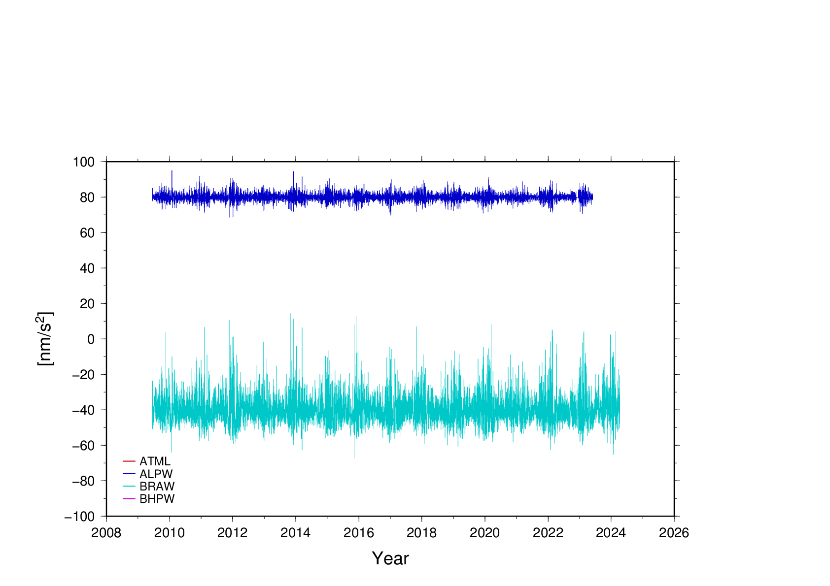
ALPW, ATML, BHPW, BRAW - A... = Atmacs time series, oversampled to 1 Sph using Fourier interpolation , B... = derived from local barometer.
ALPW: Low-pass Wiener filtered, filter determined from a low-pass filtered SG residual using the Atmacs series with a single admittance coefficient
ATML: Loading effect from Atmacs
BHPW: High-pass Wiener filtered, filter determined  from a complementary (w.r.t. ALPW)  high-pass filtered SG residual where ALPW series is reduced simultaneously
BRAW: The SG-residual remaining after reducing ALPW, ATML, BHPW, and tide gauge "bottom pressure" and the broad-band barometer series are used to determine a Wiener filter to account for the remaining signatures in the transfer spectrum.     
 
ERAI, ECCO - hydrology (ERAin) and non-tidal ocean loading (ECCO1) from the EOST Loading Service. Series of predicted gravity are oversampled to 1 Sph using Fourier interpolation. The long-period solar tides are removed, and specially with ECCO1, a Wiener filter is constructed from the Standard solution's gravity residual.

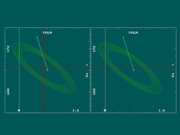
POLM - Polar motion, pure acceleration effect (expected admittance coefficient of delta-magnitude 1.16xx), computed by interpolation of IERS IAU 2000 series, file code 214, finals.data).
Despite more than 4 years of observation, the response coefficient still has substantial covariance with the annual tide parameters, see Fig. 3. We offer a long-period solution based on a 24-h sampling rate (will soon be actualized; the residual does not appear to show much noise colour, so we have avoided all pre-filtering in the 1 Spd analysis). 

ADEC, EDEC, %BS1, %BS2 ...  - The drift model, composed of two decaying exponentials. (1) with its origin at the date of installation (2009-JUN-16) and (2) with its origin at he date of repair of a feedback control unit. The decay parameters have been estimated in a particular analysis stage. Separate linear trends and offsets are associated with each exponential (%BS. =  Bias (BoxCar) and Slope). A third %BS is indicated in suit of a "rough" cold-head replacement (slope only).  Later %BS's need revision and comments.
On 2020-02-07 19:00, a spontaneous jump occurred; we estimate it as a BoxCar, symbol =UJ1.

Normalized Chi^2 of fit - The RMS of the residual (noise-whitened) is used to scale the uncertainty a posteriori. The figure would be unity if we took the degrees of freedom reduction due to the 70 parameters in the solution into account. Notice  wRMS^2 = Chi^2 in the printout.

Weff = 1.0 - the data is weighted uniformly. It could be argued that interpolation of short gaps in order to avoid longer gaps by filtering should motivate down-weighting.  

PEF: Using J.P. Burg's method, new PEF's are computed in the weekly Standard analyses and forwarded to the following week's analysis.   

1 - Decimation
We go from 1-s samples to 1-h samples with a 2-step cascaded decimation. The filters involved are symmetric. Their gain spectrum is also applied on the tide potential model. The 1-h scheme attenuates earthquakes well enough, at least those waveforms that don't cause the gravimeter's ADC to go over-range.
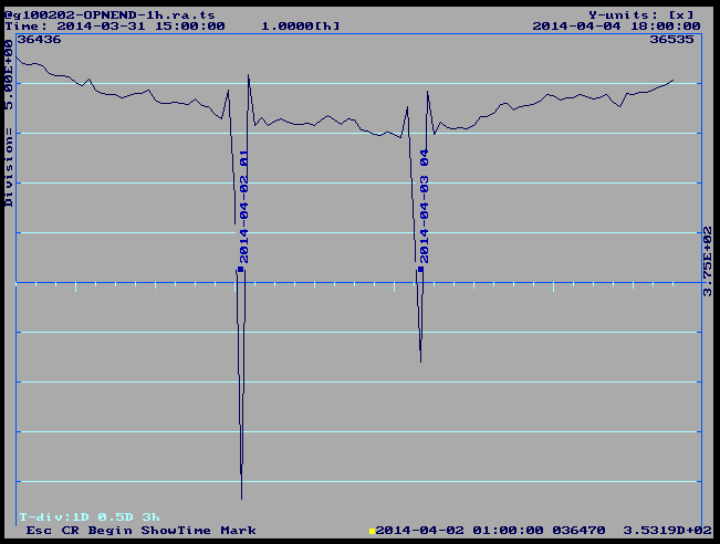
There was a strong earthquake at Tarapaca, Chile, on April 2,2014. We should inspect the gravity residual during the hours 0 to 3 a.m. that day. See Fig. 1.

2 - Tide potential amplitude and phase toning
The effects of the decimation filters on the amplitude are compensated by toning the tide potential amplitudes accordingly.
The effects of the analog GGP-filter (avoiding aliasing before ADC) are taken care of by using a numerical model of the GGP filter's transfer spectrum on the tide potential's amplitudes and - more importantly - phases. 

3 - Noise whitening:
In this strand of solution we use a simple Gauss-Markov noise model. The filter to accomplish a white spectrum is (1.0 - 0.99 z^-1)

4 - Outlier editing:
We use a criterion of 5-sigma on the not-whitened residual to delete single observations. The perturbations in Fig. 1 escape the criterion, so we have deleted them manually.

IALTG - integer - Two digits, first for radius, second for gravity
                   *0: Equatorial reference;
                   *1: IERS-definition;
                   *2: Local reference.

                   0*: Equatorial radius
                   1*: From call list: RS
                   2*: Conventional earth ellipsoid
----------------------------------------------------------------------------------

Figures

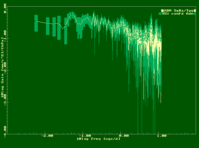
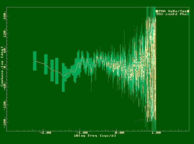
Figure 2 - Cross-spectra for gain (left) and phase (right) of gravity effect due to Kattegat. Green bars show a 95% confidence interval based on the noise level (after whitening the input), the coherence between the time series, and the degrees of freedom due to averaging and windowing (Bartlett's method, Oppenheim and Schafer, 1975).

The two time series involved have been produced in the following way. The "Kattegat-effect" (logical system input) is represented by the bottom pressure proxy at Ringhals, the sum of water level equivalent pressure at Ringhals and air pressure at Onsala (28 km distance). The gravity effect (logical system output) is computed as the sum of the least-squares residual with the Kattegat effect added back in, using the regression coefficient estimated in the tide analysis (0.0857 ± 0.0016 nm/s2/hPa)