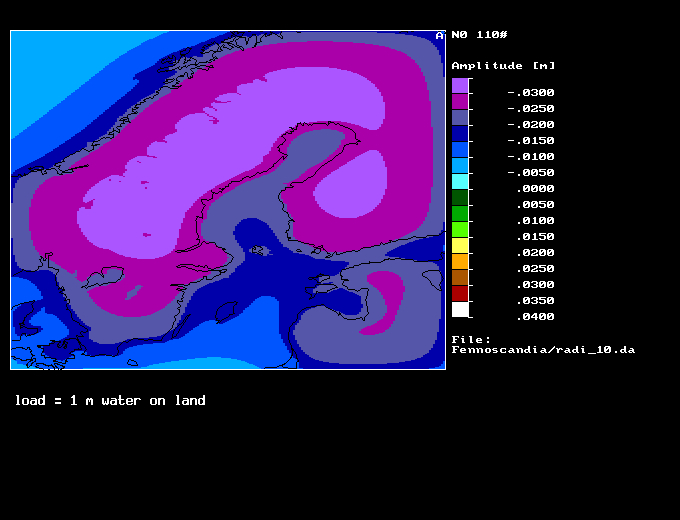
In order to obtain a first account on the order of magnitude of loading effects due to seasonal hydrological variations I have constructed a plain-grid loading model. I use Farrell's elastic Greens functions and fast convolution by 2-D Fourier transform.

The grid is 218x339 in size, 5x5 km resolution. It distinguishes the following categories of loading

1. Open ocean. Not used here (assumed negligible seasonal change as regards loading. Remember: BIFROST standard analysis is with ocean tidal loading.)
2. Land. Loading due to varying soil water saturation and snow. See Fig. 4 below.
3. Baltic Sea and its sub-basins. Seasonal water level variation is within plus-minus 0.5 m
4. Great lakes (Vänern, Vättern, Hjälmaren, Mälaren, Siljan, Storsjön), natural lakes with water level changes of 1 to 2 m.
5. Medium size lakes incl reservoirs for hydropower. Some with enormous water level variations. Due to the grid resolution the area is probably misrepresented (too large in the model).

(ftp://gere.oso.chalmers.se/pub/hgs/4jld/N0.jpg)

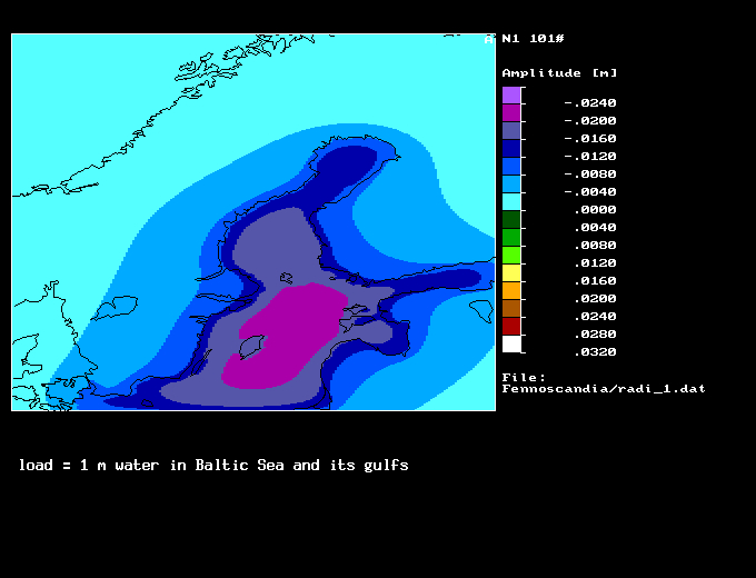
(ftp://gere.oso.chalmers.se/pub/hgs/4jld/N1.jpg)

(ftp://gere.oso.chalmers.se/pub/hgs/4jld/N3-4.jpg)

(ftp://gere.oso.chalmers.se/pub/hgs/4jld/hydro.jpg)
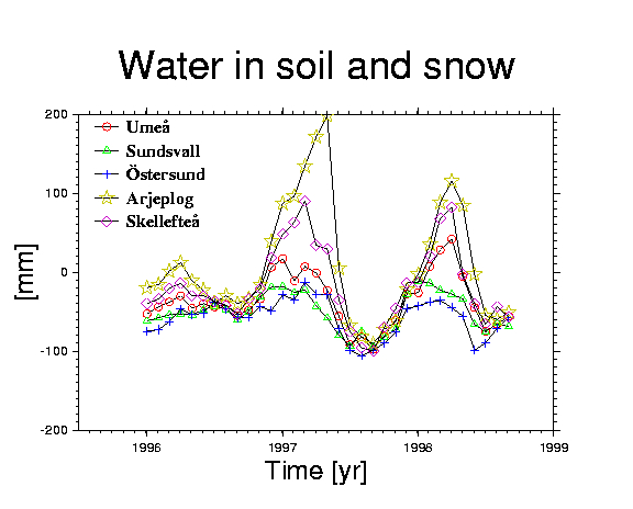
This figure represents data of five out of about 100 climatological observing stations. Daily samples of soil water undersaturation (U) and the meltwater equivalent of snow (S) measured as the height of the water column in millimetre are available. I have taken monthly values only (the snow cover might change a lot during a month, but most of the water would remain in the area) and show the combination S-U.
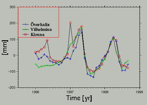
To infer the loading deformation multiply by -0.02. Thus between late spring and early autumn 1997 in Arjeplog we would expect 5 mm of uplift. You also realize the dry summer of 1997 by a deficit of 30 to 50 mm of water as compared to 1996 and 1998. Less in magnitude than I had expected and with a limited temporal extent. There is a new picture for Kiruna and Vilhelmina:

( ftp://gere.oso.chalmers.se/pub/hgs/4jld/hydro.jpg )

... and for six places in southern Sweden

(  ftp://gere.oso.chalmers.se/pub/hgs/4jld/hydro-s.jpg  )
 

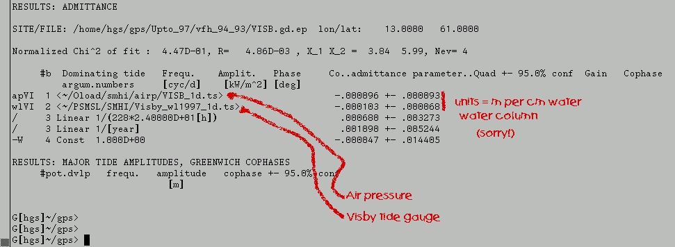
Air pressure and Baltic Sea loading
Something else: I had a look at the short-term (day-to-day) impact of atmospheric and Baltic Sea loading on Visby. First the result from the linear fit:

(ftp://gere.oso.chalmers.se/pub/hgs/4jld/VISBPRL.jpg)
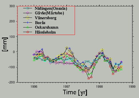
Time series were confined to 15-Jan-1997 through 31-Aug 1997. Air pressure data is interpolated fro ECMWF global files (grid interval ~1x1 degrees).  Here is the corresponding graphics, red curve shows best fit combination of sea level and air pressure using the admittance coefficients from above.

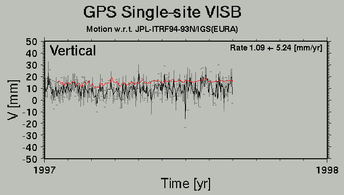
(ftp://gere.oso.chalmers.se/pub/hgs/4jld/VISB.jpg)

I find noteworthy: (1) The admittance of water level and air pressure are practically in a 1:1 relation (remember: Bottom pressure is water column + atm. press, also 1:1). The loading admittance based on the model above is 0.0002 m/cm (sorry! for the units) while we obtain half of that from the GPS analysis. The loading on the land is not sensed. We have a couple of reasons to explain the low empirical admittance, our favourite is that satellite orbit computation does not apply atmospheric loading correction, therefore orbits are slightly displaced and the the barometric loading effect is thus attenuated from range between the ground and the computed satellite position. At least in the vicinity of tracking stations. And in Europe you are always close to a tracking station if you are as large as a (anti-)cyclone.
Anyway, this was the largest admittance to air pressure and similar loading found so far in  BIFROST.