Kattegat loading
Around mid Novmeber 2009 there were a couple of sea level variations in
Kattegat, outside our door. The Superconducting Gravimeter did show
clear responses to the water level. We show that in the following
graphic.
How the data was prepared:
Gravity:
Gravimeter observations were down-sampled from 1-min to 1-hour.
An empirical tide was subtracted.
Atmospheric attraction and loading was subtracted using a single,
empirical coefficient on barometric pressure.
Tide gauge:
Tide gauge data from Ringhals (13 km to the South) was retrieved from
GOOS / SEPRISE (origin: SMHI)
Atmospheric pressure was added to water head pressure as a proxy for
sea loading.
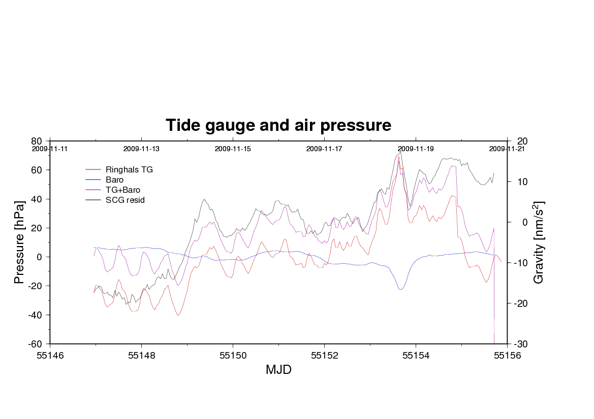
Unfortunately, the 30 nm/s2 increase during the period is
not explained by neither air pressure nor water level. Since the period
brought in quite some rain, we have to look closer into the hydrology -
an eternal and forthcoming issue.
Thanks to SMHI providing us with 7 weeks worth of Tide gauge records
from Ringhals sampled at 5 minutes rate, we can present the gravimeters
response to these sea level variations.
First, we computed the static response using a least-sqares fit of
1: TGGR = tide-gauge Ringhals plus barometric pressure at Onsala (a
proxy for bottom pressure), which is a little dirty pair;
2: BARO = barometric pressure at Onsala
to
3: GR = gravity minus tides minus atmosphere minus drift
------------------------------------------------------------------------------
Signal # <file name>
Admittance
Std.Dev.
[nm/s2 / hPa]
------------------------------------------------------------------------------
TGGR 1
<~/Ttide/SCG/o/Ringhals-wg.ra.ts>
0.023423 ±0.004237
BARO 2
<../d/G1_3_091001-300s.ts>
0.052106 ±0.041781
------------------------------------------------------------------------------
Rescaled for your convenience: For every metre of Kattegat sea
level increase we see an increase in gravity of 2.3 nm/s2
(18% std.dev.)
A residual air pressure effect is detected at 0.05 nm/s2 per
hPa, to be added to the regression coefficient of -3.488 ±0.025 nm/s2
per hPa, the one that was applied in the generation of the GR set.
The uncerntainties are with respect to an a-posteriori white noise
spectrum. White noise in the GR series was accomplished by a MEM
prediction-error filter of order 19 (Maximum-entropy method).
The spectrum characteristics of the TGGR-GR pair are shon in the
following figures.
(tomorrow!)
We can also determine the step response and the impuls response. From
the latter, a Wiener information filter will be constructed.
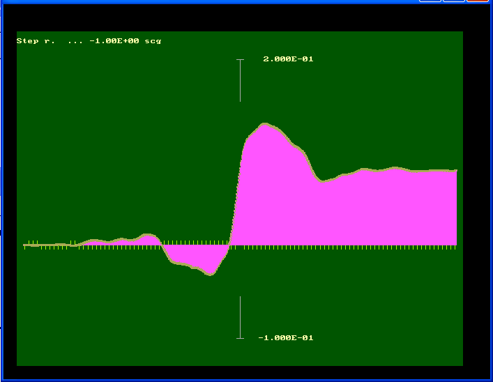
Figure 2 - Step response of the gravimeter to sea level increase at
Ringhals, units of nm/s2 per hPa (~ per cm)
A lag interval corresponds to 5 minutes of time.
The step response shows a larger amplitude than the static regression
coefficient. Here we find
13 nm/s2 per meter water level after 8 dt = 40 min,
saturating at 8 nm/s2 /m after 125 min. Notice the
anticausal
part of the response in the left half-plane (A straight-forward
interpretation would be: Ninety minutes before
an increasing event at Ringhals there is typically a low-water
precursor in the vicinity of Onsala.
2009-Nov-22 Hans-Georg Scherneck