Daily signature

Does the instrument record a "human tide"? Is there a disturbance that repeats with the working day?
To this end, I have taken the daily residuals, shifted them to synchronize with the Central European clock (daylight time from the last sunday in March to the last sunday in October), and distinguished holidays and weekends from ordinary working days. The labour-free days comprised one month of summer vcations in July and he period from Dec. 23 to Jan. 7. The two categories of days have been stacked after each day has been low-pass filtered and down-sampled to 1-min intervals. Here's the result:

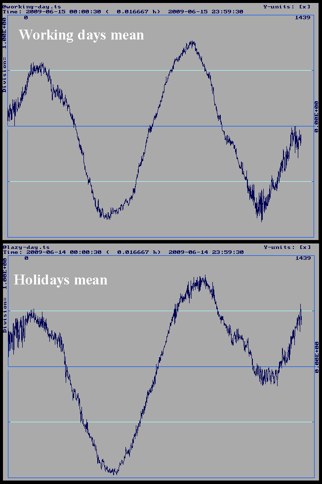
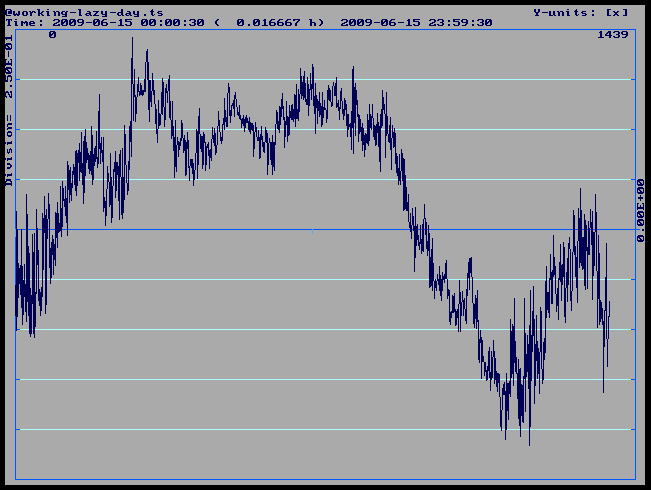
Difference working day - holiday


Units: 1 nm/s2 between horizontal lines (left), 0.25 nm/s2 (above)
Time from midnight to midnight CET(S), 1-min intervals

Conclusion: Except for a residual S2 signature (which will be investigated further, whether it is hinting at a nonstationary solar signal (a barometric tide ?!)) I do not discern a particular effect at 8-9 a.m. nor at lunch time nor between 4-6 p.m.


Noise spectrum


Here we present a noise spectrum composed of 1-second and 1-minute data.
The 1-s data covers 2010-JUN-08, a particularly quiet day.
The 1-min data stretches from 2010-JUN-08 through -18. One earthquake on 2010-JUN-12 20:20 had to be edited out (delete and interpolate).


The blue bands are (so far rather bad) renditions of the 95% confidence interval of the estimator. It is produced with a Maximum Entropy method, while the white line shows a Bartlett power spectrum (a nonparametric method using a fast method to estimate a windowed auto-covariance; here we compute 2048 spectral bins, using a 2048-taper Kaiser-Bessel window on 14336 samples). The dB units are relative to  1 (nm/s2)2/Hz.

 
The result for the MEM gets a little better when a 100-samples prediction-error filter is used insead of the 16 samples used above.


The slope that extends to 0.1 mHz is a consequence of air pressure variations. In the next graph we subtract air pressure with a coefficient of -3.4 nm/s2/hPa


If the noise between 0.01 and 0.1 mHz is still correlated with barometric pressure variations, we are inclined to believe that the transfer function is more complicated than a single, stationary coefficient. The reduction coefficient was estimated from a one-year long time series at 10-min sampling interval, so it is more represenatitive for the long-period end of the transfer spectrum.

An alternative method to show the variance in a spectrum is to plot a frequency-amplitude histogram. Like the following pair (left lin-log, right log-log)

With this method a few outliers (earthquakes?) were found, so that the noise floor could be lowered by editing out 2 samples.
The figure combines 43 periodograms, each from a 12h-wide HANN window of 60s data, shifting the window forward in time by 6h
The program used is called rastersp.f. HGS did it. Output is piped into a GMT assembly line for graphics:

foreach i ( `fromto 0 43` )
@ s = $i * 6
tslist d/gar-60s.mc -qqq -E1,2:pdgram.tse,HDW -qqq -L'G|R' -ML3.156,1,a:'B|V],Rwd' \
       -N1p,e12.4 -n/12 -sfh${s}.0 -F1p,2e12.4 -w o/gar-60s.${i}.pdg

end

cd plot

set td="2010-06-08 -19"

rastersp  -x0,30,50 -y-50,50,100 -w ../o/gar-60s.raspdg.pdg -R40 \
          ../o/gar-60s.??.pdg

xyz2grd   ../o/gar-60s.raspdg.pdg -G../o/gar-60s.raspdg.grd \
          -I0.6/1.00000 -R0.0000E+00/3.0000E+01/-5.0000E+01/5.0000E+01

psbasemap -R0.0000E+00/3.0000E+01/-5.0000E+01/5.0000E+01 -JX5/5 \
          -Ba5f0.5:"Frequ. [cyc/h]":/a20f10:"[dB]"::."Periodogram $td":WeSn \
          -K -X1.5 >! gar-60s.raspdg.ps

grdview    ../o/gar-60s.raspdg.grd -Crastersp.cpt -JX5/5 -T \
           -O -K >> gar-60s.raspdg.ps

psscale   -D5.5/2.5/5.0/0.5 -Ba0.1f0.01 -Crastersp.cpt \
          -O >> gar-60s.raspdg.ps

echo ready: gar-60s.raspdg.ps

& mutatis mutandis for the log-log diagram
rastersp  -x-1.5,1.5,50 -y-50,50,100 -w ../o/gar-60s.raspdg.pdgl -R -L2. \
           ../o/gar-60s.??.pdg

etc.


Here's the same for 10s data:

Uups! I forgot to adjust the power for the Hanning window

Here I present the spectrum of a particularly quiet day, March 17, 2010, from 1-s data:

The little spike slightly below 30 cyc/h (log f = 1.45) is a internal oscillation of the sensor ball in the confining magnetic field.
0 dB power is 1 (nm/s2)2/Hz

.bye