We have a cycleslip subroutine directly callable from tslist
(not: tsfedit).
#
# It can solve cycleslips in a time series by
# (1) improving the correlation to 1...m parallel time series
# (2) decreasing the variance of the series suspected for cycslips.
#
# Example AG drop residual and seismograph 3-D 100Hz data
# Z: sax
# E: svE N: svN
#
There are basically two superscripts, prepare and solve
prep-cycslips-problem
solv2-cycslip-problem
Prepare
The tasks are
(1) Provide the seismograms and their mutual correlations
(2) Set parameters
Before you know anything, the size of the cycleslip must be guessed:
set csize = 10.0 #
[uGal]
The strategy must be guessed (the T=-string):
source
prep-cycslips-problem sax raw SN T=0.0+S=1e10+W=0.25
(The "raw" means we prepare a job for the first time. We could
recycle a cycslip solution, but this is done in a different way now)
The seismograms need preparation. Consult ~/Seismo/gcf/HOW.TO-gcf4ag
before you execute prepare.
You need a drop residual, which is the difference between
AG-measurements and Superconducting gravimeter.
To obtain seimograph channel cross-correlation
foreach ca ( E N Z )
foreach cb ( E N Z )
foreach ka ( sax sv )
foreach kb ( sax sv )
source any-any-corr
$ka $ca $kb $cb 0 0
end
end
end
end
There are a number of default parameters in prep, of which you need
to be aware of.
Solve
Here's the logic:
- (1) Remove drift and, (2) if you have any, cycleslips,
from the drop residual:
-> ag-dropres-cyc Have or not have is
signalled by a C or no C
in the calling line.
- (3) Compute correlation coefficients between the seismic
channels and ag-dropres-cyc
-> saxZ-ag-CYCZEN.corr svE-ag-CYCZEN.corr ...
- (4) Compute prediction coefficients -> o/saxZ-ag-CYCZEN..prf
...
- (5) Predict ag-dropres-cyc -> solnew/prd/p.mc
- (6) Solve cycleslips in ag-dropres by maximising abs
value cross-correlation of seismic predictions with ag-dropres -
weight * rms after cycslip removal
- (7) Least-squares fit of predicitons to
cycleslip-resolved drop residuals
There is a range of parameters in this, so the procedure needs
iterations.
In (7) outliers are
iterated. Encircling (1) and (7), the drift parameter is iterated. These two iterations
are automated.
In (6) you need a strategy;
at least the weight factor in the penalty expression. Keyword
STRATEGY
In (5) the filter order is
needed. It's plausible with different lengths for saxZ on the one
hand and svE/-N on the other. This step can be modified to produce
predictions for a range of filter orders. Keyword MULTIPLE FILTERS
In (3) a clock offset is
detected. (1)-(3) must be rerun, possibly again in a later pass, in
order to ascertain the correct offset. Keyword: SHIFT
The whole procedure depends on the a-priori cycleslip size. Keyword: CSIZE
The reduction of RMS in step (7) may be used to judge whether
prediction and cycleslip removal was satisfactory.
Hence, the iteration on the different parameters should always
include step (7).
"Raw solution"
set prev_agdrift =
`get_prev_agdrift`
fetches the drift parameter from solold/ag-postlinpred.prl by
default.
set seishifts = ( +005 +005 )
source
solv2-cycslips-problem D
check the correlation offsets. The Z.correlogram should peak at lag
0. If not, enter S (makes solve stop), compensate by setting
seishifts accordingly and rerun
If o.k., enter G
If you're sure the shifts are o.k., run next time with
source solv2-cycslips-problem DG
If you want to fix the drift at the SG value, use
source
solv2-cycslips-problem DGU
Stepping through filter lengths:
Make the predicted series
source predict.env M
Analyze; either run with
source
solv2-cycslips-problem DGM[U]
or (edit/study the superscript and) run
cycslips-urtap-superscript
employing
cycslips-urtap.env in a loop (the subdirectory where
the urtap-prt files are collected in soldir/mfo;
cycslip-urtap.env
will create it).
"Iterated solution"
source prep-cycslips-problem
sax 0 SN T=0.0+S=1e10+W=0.25
source
solv2-cycslips-problem DG[U]
Plots
Generated on the fly: solnew/plot/ cross-correlations and linear
prediction variance
linpred-var.ps
linpred-varZ.ps
saxZ-ag-CYCZEN.corr.ps
svE-ag-CYCZEN.corr.ps
svN-ag-CYCZEN.corr.ps
Histograms:
script: source
./histogramplot
result in solnew/plot/postlinpred.ra-h.ps
Analysis of filter length
The data files are urtap protocols from which the post-fit RMS is to
be extracted and plotted versus e.g. filter lengths
The E,N-lengths on the one hand (they are supposed to be the same)
and the Z-length as the X- and Y-variables against the postfit RMS
or the RMS gain (post/pre) by colour.
Prerequisits: source predict.env M and cycslips-urtap-superscript
set anyprl = `ls solnew/mfo/c$csize-* |
head -1`
set prerms = `awk '/preRMS/{print $2}' $anyprl`
set stratmsg = "Strat.: T=0.0+S=1e10+W=0.25"
set slipmsg = ", Cycleslip = $csize"
awk -v p=$prerms '/PostRMS/{print
$4,$6,p/$2}' solnew/mfo/c$csize-*.prl >! rmsgain-lh-lz.xyz
awk '/PostRMS/{print $4,$6,$2}' solnew/mfo/c$csize-*.prl >! rms-lh-lz.xyz
makecpt -Chaxby -T#datamin/#datamax/#datastep >! rmsgain.cpt
makecpt
-Chaxby -T#datamin/#datamax/#datastep >! rms.cpt
set xl=10 xu=70 yl=5 yu=55 xs=a10f1 ys=a10f1
set xtit="Pred.Filter Length E,N"
set ytit="Pred.Filter Length Z"
set psout = $plot/rmsgain-lh-lz.ps
pscontour rmsgain-lh-lz.xyz -X2 -Crmsgain.cpt -JX6/6 -R$xl/$xu/$yl/$yu -I \
-B${xs}:"$xtit":/${ys}:"$ytit"::."RMS gain vs
PFL":WeSn -K > ! $psout
psscale -D6.5/2.5/5/0.5 -Ba0.1f0.01 -Crmsgain.cpt -O -P -K
>> $psout
pstext <<EOF -N -O -R0/1/0/1 -JX6/6 >> $psout
0.98 1.02 12 0 0 3 Strategy: $stratmsg$slipmsg
EOF
set psout = $plot/rms-lh-lz.ps
pscontour rms-lh-lz.xyz -X2 -Crms.cpt -JX6/6
-R$xl/$xu/$yl/$yu -I \
-B${xs}:"$xtit":/${ys}:"$ytit"::."RMS vs PFL":WeSn -K
> ! $psout
psscale -D6.5/2.5/5/0.5 -Ba0.1f0.01 -Crms.cpt -O -P -K
>> $psout
pstext <<EOF -N -O -R0/1/0/1 -JX6/6 >> $psout
0.98 1.02 12 0 0 3 Strategy: $stratmsg$slipmsg
EOF
Analysis of cycslip size and weight
cycslips-urtap-cw-superscript
awk '/Var-weight/{w=$6} /preRMS/{p=$2;c=$3} /PostRMS/{o=$2;print
c,w,p}' solnew/moo/*-f023-023-035.prl > ! varcw-prerms.xyz
awk '/Var-weight/{w=$6} /preRMS/{p=$2;c=$3} /PostRMS/{o=$2;print
c,w,o}' solnew/moo/*-f023-023-035.prl > ! varcw-postrms.xyz
awk '/Var-weight/{w=$6} /preRMS/{p=$2;c=$3} /PostRMS/{o=$2;print
c,w,p/o}' solnew/moo/*-f023-023-035.prl > ! varcw-rmsgain.xyz
From here on, the text is old
We use the AG drop residual which is common in each saxdata or
svdata file. We could also use
svdata/ag-dropres.ts (no label)
# Find optimum cycle slip size, weight, threshold (always "weak
strategy"):
vary-cycslips DCWPPP -r -10,10
-n -g 30 -n -s 1e10
vary-cycslips DTWPPP -r
-10,10 -n -c 11.0 -s 1e10
vary-cycslips DCTPPP -r -10,10 -n -g 30 -w 0.2 -s 1e10
At this time we have two strategies for cycle slip determination,
strong or weak.
Strong is invoked with the option +S, e.g.
-CYCSLIP${s},-3,3,T=0.+S,O#51:cycsl-ZEN.dat
and does not merit the decrease of variance
This is a strategy string for -CYCSLIP that was used with some
success
T=0.0+S=1e10+W=0.2
# this is done with
source prep-cycslips-problem
sax raw SPPPN T=0.0+S=1e10+W=0.2
# the sampling of the slip size must be set in
vary-cycleslips hands-on
Examples that vary-cycslips may provide
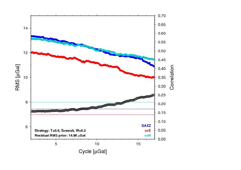
Example 1: Regularly made by prep-cycslips-problem
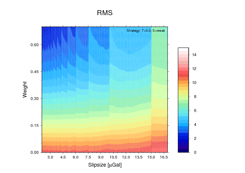
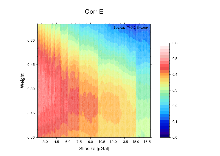
Examples 2 (left): plot/PNG/cycslip-CW-RMS-T=0.0+S=1e10+W=0.7.png
and 3 (right):
cycslip-CW-CORRE-T=0.0+S=1e10+W=0.7.png
from vary-cycslips DCWPPP -r
-15,15 -n -g 30 -n -s 1e10
provides the RMS (colour) and Correlation coefficient (abs value),
respectively, as a function of weight and slip size.
The basic ambition is to
(1) remove cycleslips to increase correlation with seismograms
(2) find a prediction filter to decrease a seismic influence on the
drop scatter; predict and obtain a residual
(3) subtract the prediction from the original series, obtain a drift
term, and go back to (1) to adjust cycleslips in those samples that
got a wrong slip
(4) when the drift term has
stabilised, subtract the iterated slip series from the original
series and compute a new prediction filter.
(5) obtain the residual and plot histograms: (a) The original
series minus the predicted seismic effect, (b) the residual, (c)
the original series minus the cycle slips.
The process is divided into three parts
(P1) Compute the corss correlations between the different
seismic channels: svE-svE-gm.corr ... saxZ-saxZ-gm.corr
using any-any-corr
(P2) Prepare = find out a viable set of csize, weight and threshold
= strategy
using prepare-cycslips-problem
(P3) Solve
using solve-cycslip-problem
The solve-stage iterates
the drift parameter and produces a time series of slips. Solve
should be iterated, since the particular
slip series will have an
effect on the prediction filter. In the next round, we use the
predicted series to - hopefully - make the slip
events better detectable.
By iteration, we hope for a convergence of the slip series and the
prediction filters.
For (P2) and (P3) there is a superscript which steps through a range
of slipsizes
#!/bin/csh
foreach
csize ( 8.0 8.5 9.0 9.5 10.0 10.5 11.0 11.5 12.0 12.5 13.0 )
source
prep-cycslips-problem sax raw S T=0.0+S=1e10+W=0.2
source
solve-cycslips-problem $1
foreach
vnr ( 0 1 )
source
prep-cycslips-problem sax $vnr S T=0.0+S=1e10+W=0.2
source
solve-cycslips-problem $1
end
end
exit
Use
superscript DH
where D requests recomputation and H histograms. The strategy is
hard-wired
(P1):
The following five jobs are needed:
source any-any-corr sv N sv EN
-005
source any-any-corr sv E sv EN
-005
source any-any-corr sax Z sv
EN -004 -005
source any-any-corr sv E sax Z
-005 -004
source any-any-corr sv N sax Z
-005 -004
source any-any-corr sax Z sax
Z -004
The pre-requist that this all works is detailed in
~/Seismo/gcf/HOW.TO-gcf4ag
(We should have it as an html)
(The prep-and-solve steps need detailed documentation; they generate
a bunch of files in a whitful set of subdirectories)
.bye