21 ^ ${EXPFIT_INPUT} Input, ts-file, reduced for tides, polar motion, atmosphere....
31 < div/rm${EXPFIT_OUT}.ts Output, prediction
32 < div/rr${EXPFIT_OUT}.ts Output, residual
33 A ${EXPFIT_TSE} Output, TSF EDIT commands for drift synthesis
41 * < div/rvar_${EXPFIT_OUT}.mc Output, IUMCV=41, variation of parameters by permutation
42 < div/reig_${EXPFIT_OUT}.mc Output, IUMCE=42, variation of parameters by eigenvectors
51 < div/rt${DT}.pef Input, PEF-bank
52 < div/rrf${EXPFIT_OUT}.ts Output, PR-filtered residual
q
| Parameter |
Type |
Explanation |
Default |
| ITER |
int |
Maximum number of iterations |
100 |
| GTOL |
real*8 |
Solution error tolerance |
1e-10 |
| P(NMP) 2) |
real*8 |
Initial values; how many need to be set
depends on size of problem. Smallest possible: 4 For every exponential and for every step-feature two additional parameters need to be set p(1), p(2) relate to initial bias and slope p(3), p(4) to first exponential. From there on it depends whether there is another exponential: p(5), p(6) Then, there is place for five more steps, either from p(5), p(6) etc. or from p(7),p(8) etc. |
|
| PVAR-START(NMP)
2) |
real*8 |
Initial variation of P() for the
iteration of standard deviations, one parameter at a time
|
|
| EPS |
real*8 |
In the iteration of standard deviations
(by bisection), the convergence parameter, which is the
difference of the penalty function of the previous two
iterations |
1e-3 |
| INPUT_MEASURE |
char*16 |
Input data unit |
'V' |
| CAL |
real*8 |
Calibration coefficient, nm/s^2 |
-776.014 |
| NEND |
int |
Cut input data at NEND |
NMAX1) |
| DEL_P(NMP) 2) |
real*8 |
In the section on eigenvalue solution to
error covariance, the variation of a parameter for
calculating the Jacobian. The formula is p' = p × (1 + DEL_P) |
all 1.d-4 |
| IUMCV |
int |
If IUMCV > 0
and a file unit IUMCV is open, output the time series
pertaining to a permutation of varied parameters. Can only be used when number of parameters is 6 or less. |
0 |
| IUMCE |
int |
If IUMCE > 0 and a file unit IUMCE is open, output the time series pertaining to the eigenvalues / eigenvector-derived variations of P(). Those of the smallest eigenvalue are suitable for an error bound of the predicted drift | 0 |
| N_PEF |
int |
Order of a Prediction-Error Filter that
whitens the input noise. If N_PEF = -1, no PEF will be
used. If N_PEF=0, a trivial PEF is used (e.g. to test the
program behaviour). If N_PEF > 0, a file with a PEF
bank must be open on unit 51. |
|
| CONFID |
real*4 |
Confidence level for parameter
covariance, Chi^2 distribution |
0.95 |
| SCLDP |
real*4 |
Scale CONFID up with this factor |
1.0 |
| IDATE(3), IHMS(4) |
int |
Date and time of first step, Year, Month,
Day...Millisecond |
|
| IDATE_EXP(3) IHMS_EXP(4) |
int |
Date and time of first exponential. Year
must be > 2000, otherwise feature will be ignored. |
|
| IDATE_SECOND_EXP(3) IHMS_SECOND_EXP(4) |
int |
Date and time of second exponential. Year must be > 2000. | |
| IDATE_x_STEP(3) IHMS_x_STEP(4) |
int |
where x is
SECOND, THIRD, FOURTH, FIFTH, SIXTH; start with SECOND and
extend as needed Dates and times of later steps. Year must be > 2000, otherwise feature will be ignored. |
|
| Remarks |
|||
| 1) |
NMAX |
Time series max. length. Defined in
~/tap/p/expfits.fp |
|
| 2) |
NMP |
Maximum number of parameters. Defined in ~/tap/p/expfits.fp |
The smpl strategy ignores
- Kattegat luni-solar tides in the water level: They will be picked up in the tide coefficients.
- Kattegat response to air pressure: The coefficients for water level and barometric pressure account for the superposition.
- Regional atmosphere effects: The Atmacs series does not cover the entire period. More important to have a consistent signal model.
The smpl strategy includes
- Polar motion in-phase and cross-phase.
- Nodal tide.
- A preliminary drift model: It will be added back to the residual and provide the input to expfitbm.
The plan for the next drift solution (prospectively mid 2017: Include -1h-files
- ECCO2 non-tidal ocean loading ( ~/TD/jpb-oce/HOW.TO )
- ERAin hydrological loading ( ~/TD/jpb-hyd/HOW.TO )
- Atmacs does cover the entire period:
Local+Regional in lm/os2009_lm2_12km_13deg.grav ,
global in ./orig/gm/*.grav
eventually append more recent series.
| We assume that the power
spectrum of the SCG noise is more flat at periods longer
than 5 days. That it can be whitened with a short PEF. Make a short, dt = 5 days series cd ~/Ttide/SCGIf you want to start 2009-06-15 you have to get Ringhals from that date. Append /home/hgs/SMHI/o/tgg-rin-100301.ts cd ~/SMHIAppend Polar Motion series: cd ~/Ttide/SCG Append the input data source urtap-openend-smpl.insAppend (re-calc) the nodal tide series: cd ~/TDRun urtapt: cd ~/Ttide/SCG Composing the input series to expfitbm: Add drift back into residual. If the preliminary drift model given to urtap was not precise, esp. concerning the decay time parameter, expfitbm will improve it (that's its purpose). setenv FNSUB o/g$startd-OPNEND-1h-smpl.ph03.tsAt the start in June 2009, there is a short linear drift term; too short to spend much effort on determination. lpf.tse,SLOPE provides a hird-wired correction: tslist o/g$startd-OPNEND-1h-smpl.ra.ts -Esubts.tse,ADD -Elpf.tse,LP1DR -Elpf.tse,SLOPE -I -o tmp/tmp4drift-1d.tsExtract the interesting date range: tslist tmp/tmp4drift-1d.ts -Bc$begdat -U$enddat -I -o ~/TD/div/ra+ph03$begdm-1d.tsRun expfitbm: setenv EXPFIT_INPUT div/ra+ph03$begdm-1d.tsMake a PEF from the residual (Example is for 1-d data): setenv DT -1d and re-run expfitbm |
awk '/TSF EDIT EXP/&& \!/TSF EDIT EXPM/{p="";qp=1;qq=0} \2. Use the new relaxation parameters in a rerun of urtapt. Set the environment parameters with
/TSF EDIT EXPM/{q="";qq=1;qp=0} \
(qq){q=q"\n"$0} (qp){p=p"\n"$0} /END/{qp=0;qq=0} \
END{print p; print q}' ${EXPFIT_TSE} >! div/expfit-sel.tse
setenv ADECAY `awk '/MAPPED/&&/EXP1 DELAY/{print $5}' expfit-2xpef-1d.log`Re-iterate the whole monty from "Run urtapt" to this point.
setenv EDECAY `awk '/MAPPED/&&/EXP2 DELAY/{print $5}' expfit-2xpef-1d.log`
cd ~/TDUse it e.g. in AG super-campaign:
set bdate=`tslp2d -, F ~/Ttide/SCG/o/g090615-OPNEND-1h-smpl.pa.ts`
set ndata=`tslqn ~/Ttide/SCG/o/g090615-OPNEND-1h-smpl.pa.ts`
cp div/synth-drift-sel.ts div/synth-drift-sel-old.ts
tslist _$ndata -BH$bdate -r1. -I -Ediv/expfit-sel.tse,EXPM -D -o div/synth-drift-sel.ts
cd ~/TD/a/Allcamps/d ; ln -s ~/TD/div/synth-drift-sel.ts syn-drift.tsUp to this point, the super-script ~/Ttide/SCG/ts4expf-drift may guide you through the process.
Better however, to make a copy
cd ~/TD/a/Allcamps/d
cp ~/TD/div/synth-drift-sel.ts expfit-synth-drift.ts
ln -s expfit-synth-drift.ts syn-drift.ts
plot-expfit-resultsResult in http://holt.oso.chalmers.se/hgs/4me/ag-superc/expfit${EXPFIT_OUT}.png
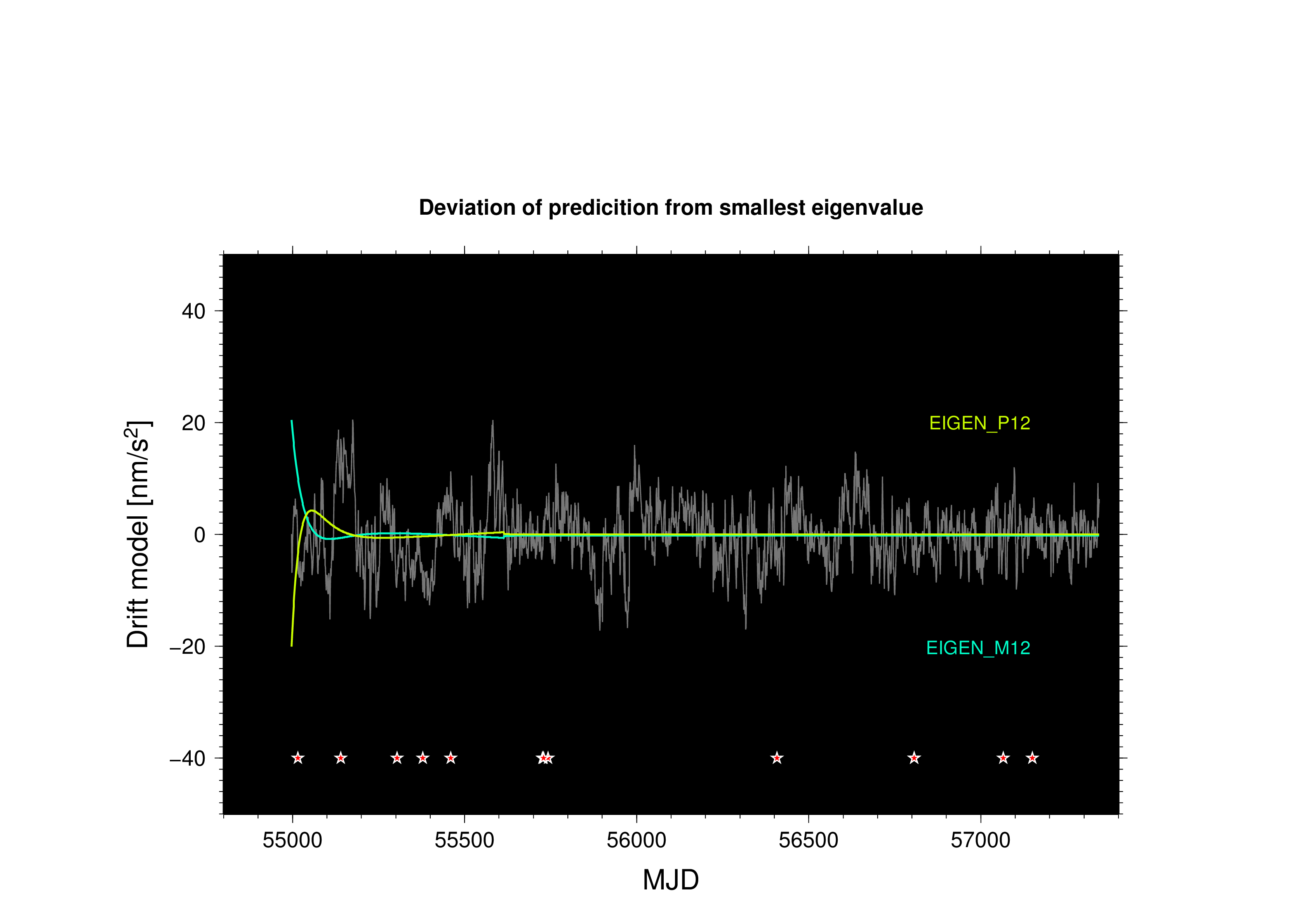
plot-varying-expfit reig EIGEN_P12 EIGEN_M12Result in http://holt.oso.chalmers.se/hgs/4me/ag-superc/expfit_reig${EXPFIT_OUT}.png
plot-expfit+devResult in http://holt.oso.chalmers.se/hgs/4me/ag-superc/expfit+dev${EXPFIT_OUT}.ps
Command
expfitbm @ expfitm.ins :2XPEF > ! expfit-2xpef.logexpfitm.ins:
2XPEF>
21 ^ ${EXPFIT_INPUT}
31 < div/rm${EXPFIT_OUT}.ts
32 < div/rr${EXPFIT_OUT}.ts
33 A ${EXPFIT_TSE}
41 * < div/rvar_${EXPFIT_OUT}.mc
42 < div/reig_${EXPFIT_OUT}.mc
51 < div/rt${DT}.pef
52 < div/rrf${EXPFIT_OUT}.ts
q
for expfitbm (bisection) (scldp was 24.)
¶m
n_pef=3
gtol=1.d-6
cal=-774.421
p= 6.131548D+02 -1.355156D+02 -7.238925D+01 -1.034555D+03,
9.754596D+01 -1.070419D+03 -8.153017D+01 1.053482D+02,
3.030403D-02 4.216255D+00 1.842617D+00 2.577364D+01
pvar_start = -100d0, -10.d0, 100.d0, 20.d0, 100.d0, -1.0, -2.0, -1.,
-1000.0, -10.0, -100.0, -10.0, -100.0, -10.0
eps=1.d-6
idate_exp=2009,06,15, ihms_exp=0,0,0,0
idate_second_exp=2011,02,24, ihms_second_exp=0,0,0,0
idate_second_step=2011,02,24, ihms_second_step=0,0,0,0
idate_third_step=2012,02,06, ihms_third_step=0,0,0,0
idate_fourth_step=2013,10,24, ihms_fourth_step=0,0,0,0
nend=99999
iter=1000, qitermon=.true.
input_measure='nm/s2'
del_p=0.01d0
varf=1.1d0, sig_d=-1.0d0, exp_sc=1.001d0
iumcv=41, iumce=42
&end
This is the status of 2016-01-08