HOW TO repair Maxwell-modes

Summary:

mode-plot →
  (cannot locate missing modes?  → maxwell for two degrees → logsd-plot )
    → maxwell for narrow s-range and high-resolution scanning
      → mode editor
         → back to beginning

Short-cut to Example 2

Detailed instructions

Example 1:
degree 124, several missed roots in the interval -0.10 < log(s) < 0.05

 run_maxwell -n 2-200 -m -s 96 0.5 10 > ! run_maxwell1.log &
The run-time parameters might have looked like
: -4.0 -1 0.0002     1.d-8
: -1    0 0.00002    1.d-8              SLC
   0    1 0.00002    1.d-7              SLC
1000 12 1.02d0 4

After the Maxwell job, create a mode plot:

ITERATION>
 cd plot

 mode-plot -H -d -dr 1e-5 10 -nr 0 201 -pr 1.e-5 10    \
          
-f ../prem_l96_um0.5_lm10.n2-200            \
           -o prem_l96_um0.5_lm10.n2-200.ps -O ~/www/4me/Maxwell/


Inspect the plot and zoom in on degrees where the fluid discrepancy is big.
 mode-plot -H -d -dr 1e-5 10 -nr 120 130 -pr 1.e-5 10    \
          
-f ../prem_l96_um0.5_lm10.n2-200            \
           -o prem-tst.ps -O ~/www/4me/Maxwell/

Maybe you can already see missing modes; note the range for s where refined iteration is needed.
If you cannot find the place, run two special maxwells for this and a neighbour degree
 ( run_maxwell -n 124-124 -m -s 96 0.5 10 > ! run_maxwell1.log ; \
   run_maxwell -n 125-125 -m -s 96 0.5 10 > ! run_maxwell2.log ) &

with the same run-time parameters!

and use (edit!)  logsd-plot-w  to run a command like
 cd ~/Maxwell
 logsd-plot -R-0.2/+0 -Y60/75 \
    -MN prem_l96_um0.5_lm10.n124-124 \
    -M prem_l96_um0.5_lm10.n125-125  \
    -IN sd/l96_um0.5_lm10.n124 \
    -o logsd-124--0.2+0.ps \
     sd/logsd_l96_um0.5_lm10.n124 sd/logsd_l96_um0.5_lm10.n125
i.e. something like
 logsd-plot-w -0.2/+0 124 125
You may have to issue many such plotting jobs.

Once you've found the s-range, run a narrow scan with a refined basic interval
Edit the second instruction block in  run_maxwell (else ... fi)
prem l=$1 um=$2 lm=$3 $4
$from $to 1
$slo $shi 0.000005    1.d-8    SLC
500 12 5.0d0 4
EOF
 run_maxwell -n 124-124 -S -nrw124 -0.1 -0.05 96 0.5 10
This job will create  prem_l96_um0.5_lm10.n124-124-nrw124
Add the roots using the mode editor
 moded @moded.ins '>124>'
with moded.ins:
124>
21 R prem_l96_um0.5_lm10.n2-200
22 R prem_l96_um0.5_lm10.n124-124-nrw124
31 B prem3.tst
   Q
INFM1 124
ADDM  124
INFM1 124
END

and check now with either
 love-list -c1.d-16 -Tir -l0,201 -f prem2.tst | fgrep Mode_sum | m
or with a new mode plot (now using file prem3.tst)


Example 2:
n=102, bad convergence for the first two zero-crossings and a missing root at s ~ 0.65

 cd plot
 mode-plot -H -d -dr 1e-5 10 -nr 65 105 -pr 1.e-5 10 -f ../prem_l96_um0.5_lm10.n2-200 -o prem-tst.ps -O ~/www/4me/Maxwell/
 cd ..
Shown in Fig. 1 below. Notice the missing modes  -4 < log s < -3

 ( run_maxwell -n 102-102 -m -s 96 0.5 10 > ! run_maxwell1.log ; \
   run_maxwell -n 103-103 -m -s 96 0.5 10 > ! run_maxwell2.log ) &

You can use
 root-iter-plot -n 1 sd/l96_um0.5_lm10.n102
or
 root-iter-list -n 1 sd/l96_um0.5_lm10.n102
to check on the convergence of the bisection:
Model:  l96 um0.5 lm10
Shd:  102
>     1    1         1       952 #quit
   1.54953003958e-04   1.75024e+00    0    1.73419e-65    2.05787e+57 ::  0         0  -3.80980000e+00
   1.55024378887e-04  -2.49759e-01    0    1.73419e-65    2.05787e+57 ::  0         0  -3.80960000e+00
   1.54988687314e-04   5.99153e-01    1    2.04308e-65 :: +1  -0.222462  -0.680084 -3.80970000e+00
   1.55006532073e-04   3.22599e-01    2    1.51522e-65 :: +1  -0.491337  -0.504374 -3.80965000e+00
   1.55015455223e-04  -5.45131e-02    3    1.14982e-65 :: -1  -1.263499  -0.382743 -3.80962500e+00
   1.55010993584e-04  -2.94543e-02    4    6.15821e-66 :: -1  -1.530851  -0.204989 -3.80963750e+00
   1.55008762813e-04   1.73149e-01    5    5.35044e-66 :: +1  -0.761580  -0.178101 -3.80964375e+00
   1.55009878194e-04   1.51538e-01    6    2.99466e-66 :: +1  -0.819478  -0.099684 -3.80964063e+00
   1.55010435888e-04   1.00449e-01    7    2.08621e-66 :: +1  -0.998054  -0.069444 -3.80963906e+00
   1.55010714736e-04  -8.86106e-03    8    1.23962e-66 :: -1  -2.052514  -0.041263 -3.80963828e+00
   1.55010575312e-04   4.35174e-03    9    5.12771e-66 :: +1  -2.361337  -0.170687 -3.80963867e+00
#quit          1    1   1.55010575312e-04  2.41749E-01  1.26117E-44 -3.80964E+00  5.12771E-66  1.23962E-66

Notice that the root search quit on large changes of the SD (notice the past tense in this sentence).
This was a mistake in maxwell.f: The slope convergence criterion was not active in this range of s, yet the quit-condition was in effect.
An ".and.qslcvcr(jj)" was missing in line 266. Corrected 2013-07-08.
However, the check with root-iter-list is revealing now that the slope still changes much in the last iteration steps. It appears worthwhile to go higher in the number of bisections although the mode strength is rather small. This is a slow mode, so in a Heaviside load event starting long ago the effect could become important. You notice the uneven magnitudes and eventually missing modes in the low-s region.

The missing root for n=102 is seen in the mode plot at high s ~ 0.65 (Figure 1, log s ~ -0.19). The region between -0.22 and -0.15 contains difficult zero-and-pole structures; the neighbour of root 266 could not be resolved. The results shown in Figure 2 are from the high-resolution scan.

I have no idea how to solve this problem. The last resort is perhaps to copy the roots from the neighbour sph.harm. degree.


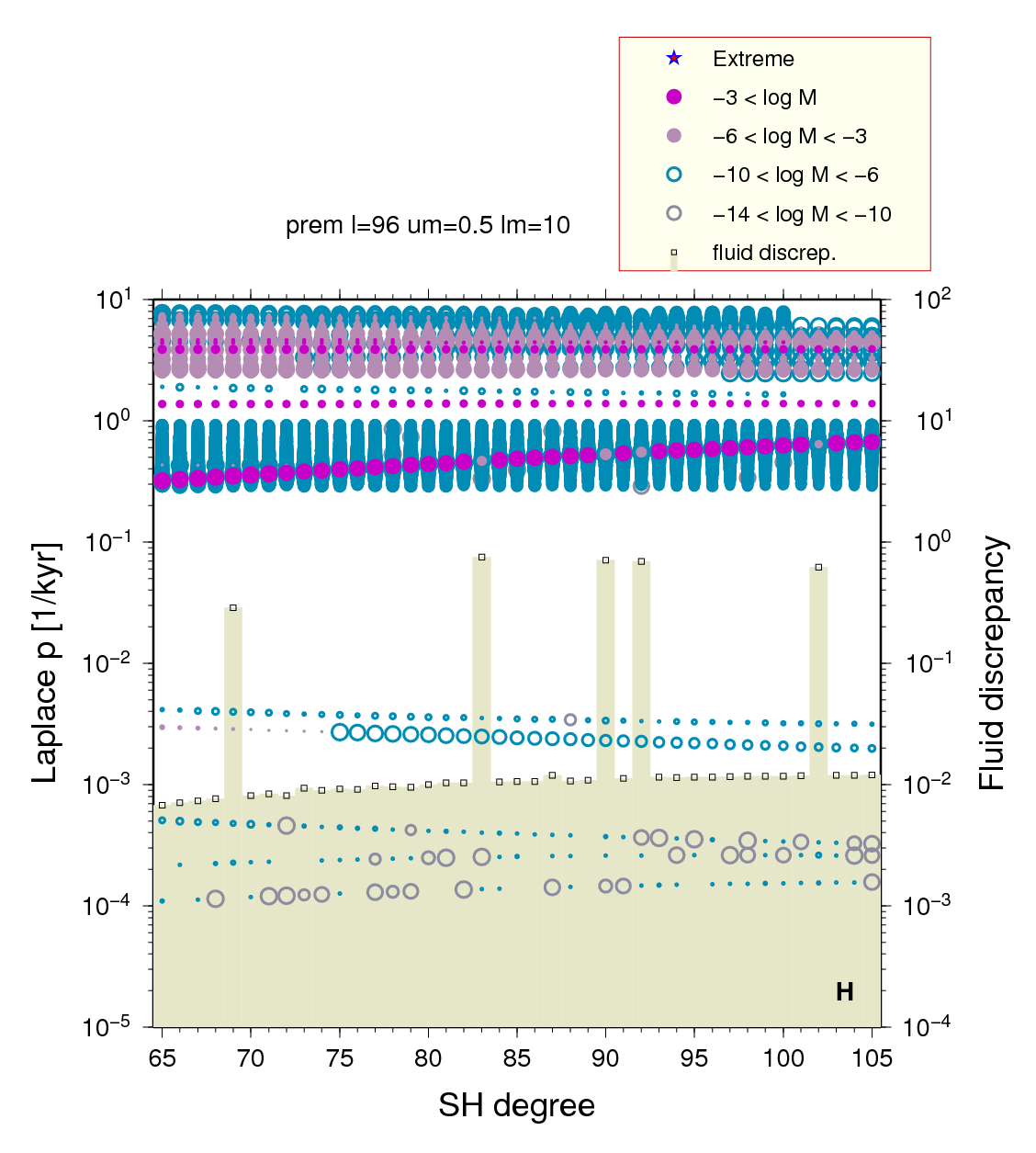
Figure 1 - Five root-finding problems. In the set with n=102 a root is missing near s=0.65 (log s ~ -0.19) (Laplace p = s, sorry!) Also note the irregularities in the low-s modes, probably a numeric precision problem. The big fluid discrepancy in the set n=69 has a different reason altogether. Click on graphics to get full-scale image.
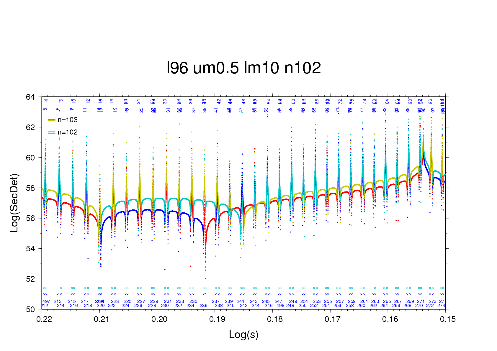
Figure 2 - The secular determinant in a narrow range 0.603 < s < 0.708. Notice that the problem of a near-zero (i.e. two red-coloured dip flanks at -0.192) does not exist at n=103. Click on graphics to get full-scale image.


Example 3:
The case of n=69

Here, the greatest root has a much different strength compared ot its nearest neighbours. We use a new tool, a plotting script that creates a time series for a Heaviside load.
  steprsp-plot 68 69 70
The script contains a call to love-list and then invokes m/steprsp.f. With the option -statF file  the latter program produces a sorted list of the contributions to the step response evaluated at the last time step, which in the present case is 10 kyr, and outputs the corresponding mode-s and strengths.
   paste -d' ' stepstat*.rsl
  3.42482960D-01     -4.79852610   3.50011200D-01     -6.45310790   3.57674990D-01     -4.69421000
  3.88344320D+00     -0.05948305   3.88392240D+00     -0.05823763   3.88440510D+00     -0.05700377
  1.37409920D+00     -0.04007524   1.37508100D+00     -0.03933680   1.37597800D+00     -0.03860817
  4.64213180D+00     -0.00175455   4.64227670D+00     -0.00166311   4.64241480D+00     -0.00157649
  4.41931800D+00     -0.00148794   4.41935590D+00     -0.00148613   4.41939880D+00     -0.00148324
  4.39796640D+00     -0.00100887   4.39795600D+00     -0.00096705   4.39794390D+00     -0.00092593
  2.63210490D+00     -0.00063406   2.63251570D+00     -0.00062369   2.63288870D+00     -0.00061196
  3.83902390D+00     -0.00059663   5.18661750D+00     -0.00052616   5.18714550D+00     -0.00047744
  5.18606730D+00     -0.00057936   3.83876670D+00     -0.00050335   2.80870000D+00     -0.00044386
  2.80857260D+00     -0.00049871   2.80863500D+00     -0.00047054   3.83852290D+00     -0.00042519
        sj                H
j            sj                  Hj             sj                Hj
  --------------- 68 -----------   --------------- 69 -----------   --------------- 70 -----------

Notice the different strength values in line 1, i.e. for the most important root! At n=69 log(s1) = -0.455918
The strength value increases with further bisections (16 instead of 12) but does not reach the typical level, order of one. Two roots and one pole are placed close together. 

The cases for n = 83, 91, 93, and 102 are similar. Here's how to interpolate:
  steprsp-plot {n-1} {n} {n+1}
  paste -d' ' stepstat-{n-1}.rsl stepstat-{n}.rsl stepstat-{n+1}.rsl
In the columns for n find the mean s where a mode is missing/underestimated from the neighbours
  calc '(3.42482960e-01 + 3.57674990e-01)/2'
0.350079

Edit the instruction file moded.ins
INT>
21 R prem3.tst
31 B prem4.tst
   Q
EPS= 1.d-3
INPS  69 0.350079
INPS  83 0.467123 ALFA=0 RADIUS=0.3
INPS  90 0.531016
INPS  92 0.549604
INPS 102 0.643244
END

  moded @moded.ins '>INT>'

check with
  mode-plot -H -d -dr 1e-4 100 -f ../prem4.tst -nr 65 130 -pr 0.1 1 -s 1 -o prem4-tst.ps -O ~/www/4me/Maxwell/

The mode editing job leading up to prem3.tst is
ALL>
21 R prem_l96_um0.5_lm10.n2-100
22 R prem_l96_um0.5_lm10.n101-200

31 B prem3.tst
   Q
NCOP 101 .. 200
INSR prem_l96_um0.5_lm10.n124-124-nrw124
ADDM 124
INSR prem_l96_um0.5_lm10.n83-83-hi83
ADDM  83
EPS= 1.e-3
END

.bye