SCG Tide analysis with whistles and bessels


Content

1. The long road to data preparation
    1. Earthquakes and other disturbances
    2. Gravity and barometric pressure
    3. Ringhals tide gauge
    4. Weights for gaps
    5. Polar motion
2. The analysis proper

3. An open-ended analysis, weekly
4. The analysis carried out in November 2013
5. The analysis carried out in March 2014


The long road to data preparation

A first analysis takes as long records as possible, meaning

  1. No Atmacs pressure loading series (we may extend the analysis by supplying Atmacs in two channels and, before Atmacs' start, local pressure in a third).
  2. No Kattegat sea level
  3. No local weather data, nothing from the borehole, ...


  cd ~/TD
  eq2wdr
...
  mc4tideanalysis ...
  weights4gaps
...
  polmotm ...
#
# Specific guidance, example is for date range 090701 - 130515
#
# There is a super-script:  ~/TD/all4tideanalysis
#
Earthquakes and other disturbances
# Irregardless of sampling rate:
   eq2wdr -t 20 -m -360,1440 -n 1415 090701
# -t 20        - 20 nm/s2 threshold (on RMS of differenced data)
# -m -360,1440 - margin for gap width around the event
#
# will create files        d/eq_YYMMDD.tse  with  DEL  statements;
# will create monthly files  o/eq_YYMM-rms-20s.ts with the IIR-filtered RMS series;
# will delete empty d/eq*.tse files at the end of the process.
# The tse-instructions are:
TSF EDIT EQ
; Note: Reasonable defaults so you can run tslist directly
;       although this section is dedicated to ~/TD/eq2wdr
;
FILTER D:WD KAIS 80 2.1 0 0.05 1.0 0.0
DECIMATE 20 ${MOVE} 0
FILTER 0 1 ' '
1.0 -1.0
MOVRMS 1 10
IIR 1
1.0 0.5
;
; This creates the event files: WDR...
OPEN 31 ${EQTSEO:[A]} ${EQTSE:[eq.tse]}
;
; You might like to use the margin option, e.g. MS=-600,600
WDR ${EQTHR:[20]} U=31 MS=${EQWDRM:[0,0]} From #0 To #4520
; 4520: we need overlap, too much doesn't hurt
; 70 minutes for 600s-data plus the 120s due to MOVRMS
; calc '(86400+3660)/20+10' -> 4513
END


Time series for tide analysis: gravity and barometric pressure:
# For 1h-data:
   mc4tideanalysis -4 -c c -wa tmp/collect.tsf -n 1415 090701
# -4        - 1h-data out.
# -c c      - re-calibrate to obtain original Volt values
# -wa file  - the collecting ascii file
#
# For 600s-data:
   mc4tideanalysis -3 -c c -wa tmp/collect.tsf -n 1415 090701
# -3        - 600s-data out.
#
# Resulting files:  d/g090701-130515-1h.mc  d/g090701-130515-600s.mc 
#

Ringhals tide gauge:
# Now that we have a barometer series, convert tide gauge to bottom pressure, TGG in cm, result in hPa:
# From scratch, get the first part from SMHI/TGG/Ringhals-2009-1h.tsf
cd ~/SMHI/TGG
tslist Ringhals-2009-1h.tsf -gi4,3i3,t20,f7.0 -BHc2009,7,1,0 -k1 -I \
-o Ringhals-090701-091231-1h.ts
# Append from the latest croned update:
cd ~/SMHI
setenv BAROFILE ~/TD/d/g090701-140131-1h.mc
setenv BAROLABEL 'L:B|V'

tslist-app -I -U2014,1,31 -o o/tgg-rin-090301-140131.ts + \
           TGG/Ringhals-090701-091231-1h.ts \
           o/tgg-rin-100301
.ts 
tslist o/tgg-rin-090301-140131.ts -Ebp.tse,B -I \
       -o ~/TD/d/bp-rin-090701-140131-1h.ts

# (the environment setting above are actually the defaults)

Weights for gaps:
# We split the jobs into two steps so we can update the constant background weight
# when we have evidence from urtap. OBS! The output weights will also be re-calibrated;
# thus, we need to specify the calibration factor also in the Downweight block to urtap.
# For 1h-data
   weights4gaps -4 -c c -A      -wa tmp/wg         -n 1415 090701
   weights4gaps -4 -C #weight c -wa tmp/wg -O d/wg -n 1415 090701
# -c c       - re-calibrate
# -A         - only the accumulation stage to ASCII
# -C         - only do the ASCII to BIN conversion
# -wa tmp/wg - write everything into one file tmp/wg_YYMMDDf-dt.tsf
#              YYMMDDf from the first day
# -O d/wg    - convert to BIN d/wg
YYMMDDf-YYMMDDl-dt.ts 
#              YYMMDDf from the first and YYMMDDl from the last day
#
# For 600s data, again, option -3 is supposed to do the change.
# Resulting files:  d/wg090701-130515-1h.ts d/wg090701-130515-600s.ts
#

Polar motion:
    cd ~/TD/d
    polmotm -l 11.9,57.6 g090701-130515-1h.mc | fgrep -v '<' |\
     tslist - -gI4,4i3,t66,f10.0 -k2 -C1 -I -U`tslq -e g090701-130515-1h.mc` \
            -E../repair.tse,R -S1.16 -o PMG090701-
130515-1h.ts

# Scale with 1.16 in case you want to subtract PM instead of solve for it.

The analysis proper

 cd ~/Ttide/SCG
 setenv URTAPFD 090701-130515
 setenv URTAPDT 600s
#
# Take the ins-file urtap-bigtidesww.ins as an example.

#
# The weights series:
# wg090701-130515-600s.ts
# Start must exactly synchronize with the observation series  d/ga090701-130515-600s.mc .
#
# Preparing the iteration:
# The procedure that iterates the solution for outliers (and renews PEF's en route) is urtap-outlit
# You start most often with an empty outlier file.
# If the namelist runs a parameter
tsfile_names='o/g${URTAPFD}-${URTAPDT}-lapww '
# The tse file must either be empty at start
  rm -r o/g${URTAPFD}-${URTAPDT}-lapww.tse
  touch o/g${URTAPFD}-${URTAPDT}-lapww.tse
# or be copied from a stub
  cp d/g090701-130515-stub.tse o/g${URTAPFD}-${URTAPDT}-lapww.tse
# urtap-outlit can do either: Specify  -f d/g090701-130515-stub.tse for copying the stub.
#
# The PEF filter can be iterated from scratch. For a starting solution, specify in namelist &param:
  lpef=0
# and reference just any PEF to open on file unit 41.
# If the result is acceptable,
  cp d/grav-600s-it.pef d/grav-600s.pef
  lpef=#order
#
# BEWARE: Automatic iteration of the PEF bears the risk of getting trapped in
# undesirable filter properties. The filter order might need change
# (dynamic use of Akaike-crit., not implemented). Better to manually
# determine a PEF with sasm03.

#
#=======================================================================
#

An open-ended analysis


The instruction file is loosely built from urtap-bigtides-rawrin.ins
The results that can be expected are not as unbiased as those from urtap-bigtides-bpfM6.ins
(which requires tide analysis of Ringhals tide gauge)

setenv URTAPFD 100202-OPENEND
setenv URTAPDT 1h


The time series subjected to / involved in /  the analysis are


21 ^ d/g${URTAPFD}-${URTAPDT}.mc            Gravity in Volt, Baro
22 ^ d/PMG${URTAPFD}-${URTAPDT}.ts          Polar motion
23 ^ d/boa-${URTAPFD}-${URTAPDT}.mc         Atmacs
24 ^ d/bp-rin-${URTAPFD}-${URTAPDT}.ts      Ringhals bottom pressure, tides not removed
30 R urtap.tse

Brainstorming:
We need a croned script that keeps the OPENEND series up to date.

d/g...ts   - find out the last date on file, append 1h-data (model: mc4tideanalysis)

Ringhals - the 1-h series is updated automatically. We only need to add 1-h local pressure data here.

Atmacs - 3-h data is updated automatically, but here we need 1-h data. This has not been covered above at all; however, see
http://holt.oso.chalmers.se/hgs/hgs.man/SCG-Data-HOW.TO.html#Atmacs
=>  ยง Atmacs interpolation with the gain method

Earthquakes and other disturbances: Big earthquakes can go into the tse-file  o/g${URTAPFD}-${URTAPDT}.tse
Smaller shocks during the most recent week will be included next week due to the outlier criterion.
Would be good to issue a prompt by cron: Please review last week's earthquake situation, add events if necessary.

Polar motion must involve an automatic download from the IERS data archive - most critical since they appear to change directories and file names quite often.
If the step does not succeed, a warning message should be issued, e.g. by email.


Analysis November 2013, 1h-data:
Since a change of drift with an initial exponential was detected, the decay time had to be estimated first.
In TD/div/ a zero-order residual was produced (1h sampling rate) ("hand-selected")
ls div/g100224-130515-1h.rh01.ts
ins4env expfitm.ins
expfitbm @expfitm.ins :BISECT
The result for the starting point and the decay time go into Ttide/SCG/urtap.tse
and the amplitude will be a parameter to solve for.
Since reduction for Kattegatt effects was aimed at, all time series have been cut to start at
2010 02 02 11, sampling interval 1h.
For the different stages in urtapt analysis there are - in succession - the following subdirs:
o/   - Ringhals bottom pressure ("Kattegatt")
on/  - No Kattegatt, estimating M6 in gravity
oa/  - With Atmacs and Kattegatt
ow/  - With weights, Atmacs, and Kattegatt
ofw/ - With weights, Atmacs, and Wiener filtered Kattegatt
olp/ - Long-period
Ringhals: urtap-ringhals.ins backup copy:  on/urtap-ringhals.ins  [sic: on/]
Except for olp/ the gravity analysis has been carried out with urtap-ev-ins ("engineeringversion").
Changes: LPEF orders, alt. DIFF filter; outlier detection on the basis of ra.ts or wr.ts
The last version has been saved in owf/urtap-bb.ins ("broad-band") and in olp/urtap-lp.ins
sasm03 @sasm03-tst1h.ins         for generation of PEFs, backup copy:   ofw/sasm03-tst1h.ins
sasm06 @sasm06-gr-tgg-1h.ins     for generation of Wiener filters, backup:   on/sasm06-gr-tgg-1h.ins
The PEFs were always created on the basis of .ra.ts
Reweighting in ~/TD with weights4gaps and tslist for cutting to the appropriate start time.

Long-period:
A reduced observation file has been prepared:
tsl d/grav-ev.mc -L'G|V' -I -Eaprestap.tse,AK -O:`label GRAV,VAL` olp/grav-ev.mc
to subtract Atmacs and Kattegatt with the best-fit coefficients from the broad-band stage.

Plot the residual+drift with
tsld olp/g100201-130515-1h-lapww-M6.rh02.ts -I + -n29000,1,c -F
Plot the drift model with
tsld _29000 -r1 -B2010,2,2,11 -Eaprestap.tse,DRIFT -I + -n29000,1,c
The tide models (.trs) have been combined:
# tt/g100201-130515-1h-lapww.trs =
# Long-period tides from olp/g100201-130515-1h-lapww.trs
# Diurnal.. tides   from owf/g100201-130515-1h-lapww.trs
A summary of numerical results with comments is in ~/Ttide/SCG/apload-results.txt

Conclusions:
The 1h-results for the period Feb. 2, 2010, to May 15, 2013, are good:
Residual min / max / ave / rms:
To use 600s data will not help to improve on  the two major problems:
1- The drift change in 2011; 2- the impact of Kattegatt water level.
Remains to show how well 1s data predicts measurements when downsampled to 60s or 600s. 

Analysis February-March 2014

Time series extended to 2014-01-31
Most complete signal model:
urtap-bigtides-bpfM6.ins
Iteration for variations of the instrument factor:
Program twotsradm (~/sas/p/mt/twotsradm.f) computes admittance coefficients.
twotsradm.ins section PT>:
PT>
 &param
 fnin_x='/home/hgs/TD/o/pt.ts'
 fnin_y='o/g090701-140131-1h-boa-bpfM6.ra.ts'
 fnout= 'o/g090701-140131-1h-boa-bpfM6-ra-adm.ts'
 repair_opt='L'
 nfp=58, fwin='KAIS', f1=1.d0, f2=2.d0, fny=12.d0, fcal=1.5d0
 lw=48
 m=1
 window='HANN'
 qsqr=.false.
 qremdc=.true.
 &end
As input we use a theoretical tide series computed by
run_urtip  -b o/pt.ts -t ~/Ttide/SCG/tt/g090701-140131-1h-boa-bpfM6.trs \
           ~/Ttide/SCGo/g090701-140131-1h-boa-bpfM6.ra.ts

Both series are band-pass filtered to retain only diurnal and semi-diurnal effects.
After
urtapt @ urtap-bigtides-bpfM6.ins > ! urtap-bigtides-bpfM6.log
we compute the admittance
twotsradm @ twotsradm.ins :PT
using a 96-hours sliding interval to compute admittance factors on an hourly basis, saved in o/g090701-140131-1h-boa-bpfM6-ra-adm.ts
The result must be imbedded in a series that starts and ends exactly concurrent with the residual:
setenv SUPPFILE o/g090701-140131-1h-boa-bpfM6-ra-adm.ts
tslist _40239 -r1. -BH2009,7,1,5 -Esupp.tse,S -I -o save-adm/adm-it0.ts
This admittance file is used in urtap-bigtides-bpfM6.ins again to tune the input. We process it in the section
TSF EDIT CLEAN
...
OPEN 51 ^ save-adm/adm-it0.ts
51,'BIN]',-99999.0,'U', 0, 0, 'K', -1.0
CLOSE 51
X*W +W=1.0
OPEN 51 ^ save-adm/adm-it1.ts
51,'BIN]',-99999.0,'U', 0, 0, 'K', -1.0
CLOSE 51
X*W +W=1.0
OPEN 51 ^ save-adm/adm-it2.ts
51,'BIN]',-99999.0,'U', 0, 0, 'K', -1.0
CLOSE 51
X*W +W=1.0
OPEN 51 ^ save-adm/adm-it3.ts
51,'BIN]',-99999.0,'U', 0, 0, 'K', -1.0
CLOSE 51
X*W +W=1.0
...
(the files adm-it1.ts etc. have been made with the same recipe in a series of runs of urtap)
An iteration loop can be programmed (source iterate-radm.env)
with a TSF EDIT CLEAN section
FMT###LOOP=i1
LOOP ${ITER:[-1]} 1 0 <101>
OPEN 51 ^ save-adm/adm-it###LOOP#.ts
51,'BIN]',-99999.0,'U', 0, 0, 'K', -1.0
CLOSE 51
X*W +W=1.0
ENDLOOP <101>
In the end we produce the product of the admittance files
tslist _40239 -r1. -BH2009,7,1,5 -Esupp.tse,A -C3 -I -o save-adm/adm-product.ts

Discussion

Figure 1 shows the product of the admittances from the iteration. The residuals are so similar to each other that there is nothing to discuss.
Taking a look at the M2 delta factors, there is a change at the 0.06 permil level.
It           Real                 Imag             Amp      Pha
0    1.193379 +- 0.0004   0.026451 +- 0.0004    1.193673    1.27
1    1.193444 +- 0.0004   0.026448 +- 0.0004    1.193737    1.27
2    1.193480 +- 0.0004   0.026445 +- 0.0004    1.193773    1.27
3    1.193487 +- 0.0004   0.026443 +- 0.0004    1.193780    1.27
4    1.193473 +- 0.0004   0.026442 +- 0.0004    1.193766    1.27
5    1.193452 +- 0.0004   0.026443 +- 0.0004    1.193745    1.27
The admittance product shows two features: An annual period and an offset.
The offset ends at the time when the pressure control unit has been repaired (2011-FEB-23). Before 2009.7 the offset does not appear to be present.
The annual periodicity, noting its small magnitude, might be explained by the wide-band formulation of the high-order tides in the analysis,
n=3 (m=0,1,2,3):  constant response  w.r.t. m is assumed,  and
n=4 (m=0-3,4): constant response is assumed over the whole range of 0 <= m <= 3

Similar magnitude of an annual periodic signature has been found in admittance of the time-derivative of the model tide (Figure 2).
That plot does not exhibit an offset between 2009.7 and 2010.2.

The similarities in the annual signatures in Fig. 1 and 2 may be another point in evidence for the suggestion of side-effects of the wave-group design.
Both plots, however, show a concurrent signature concentrated to the first two months.

The signatures are always safely inside the uncertainty of the AG-calibration efforts (0.04% vs. 0.2%)


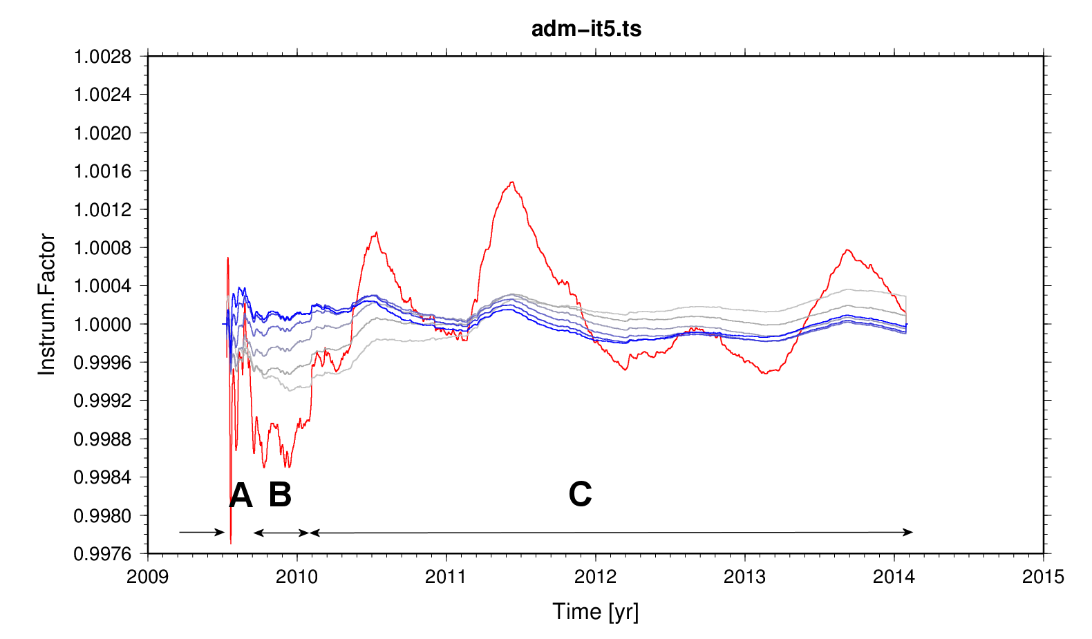
Figure 1 - Sliding-window admittance of average predicted tides w.r.t. observed tides.
Grey to blue: relative change per iteration. Red: final product. Three periods for the instrument factor can be distinguished: A - normal, B - low, C - normal again. 

The behaviour of the instrument sensitivity is not well understood. Besides the annual periodicity, which might have a simple explanation.
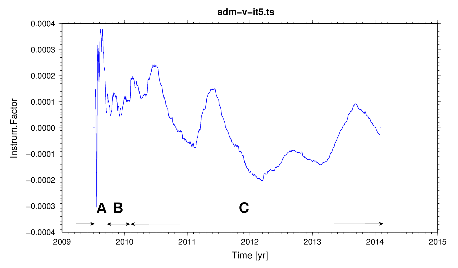
Figure 2 - Iteration 5 with the time-derivative of the theoretical tide. The annual periodicity might be attributed to wave-group design and high-order tides. Period A appears anomalous; however, consider that the annual peak in 2009 might already have been passed, and the pressure control circuit (which appears to be the reason for the lower sensitivity and, b.t.w., a profoundly different drift signature) may have started to malfunction at the beginning of period B.


.bye