grdcvem - list/plot parameter correlations after urtapt
USAGE:
grdcvem [options] eigenvalue-file.evs
OPTIONS:
-m msgfile
- open a file for diagnostic output (e.g. /dev/pts/#n)
-c corrfile - open a file
for output of correlation table.
-h
- help
Program has two tasks:
(1) Print the correlation triangle in human-readable form.
(2) Plot correlation ellipses interactively
The first task is requested by specifying both the number of frames
as -1 and the first parameter to pick for plotting as -1.
For the second task, enter e.g. 6 to prepare space for six frames on
the plotting surface, and pick an interesting parameter.
The parameters are picked by number. Read the correlation file and
find out which parameter number corresponds to which symbol.
EXAMPLE:
grdcvem -c tt/urtap.pcorr -m /dev/pts/6 tt/urtap.evs
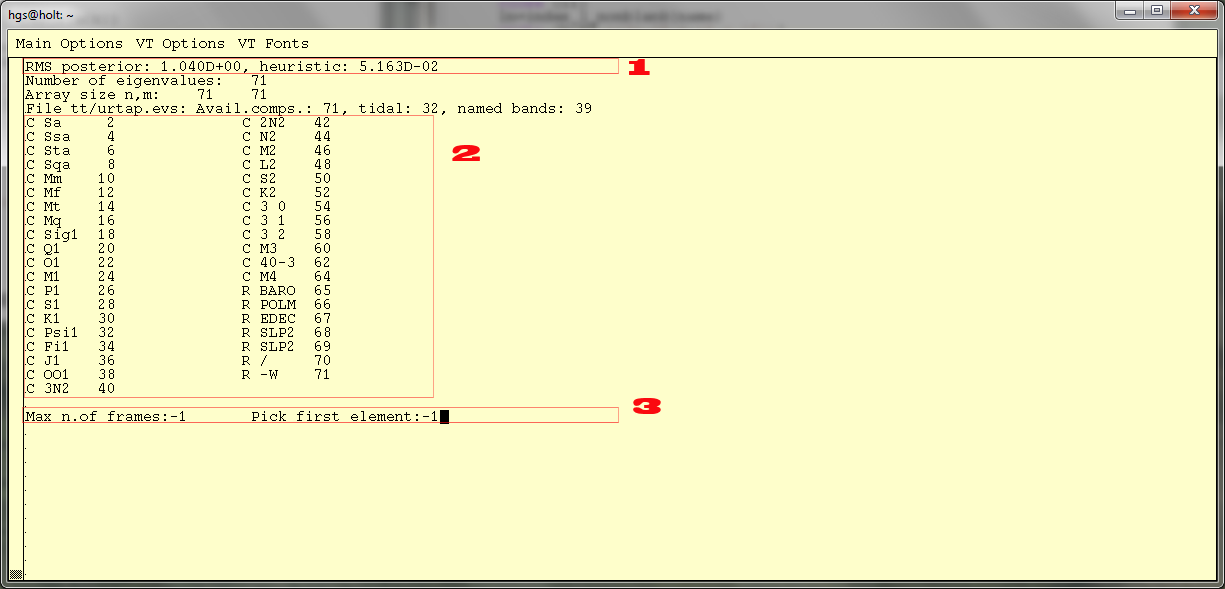
Figure 1 - Do task (1) only. At "1" the a-posteriori RMS is shown
("q_hindsight=.true." in urtapt). That job used down-weighting, and
the a-priori weights have obviously been too big. Since there is
little means to scale the weights realistically in advance, the RMS
result is characterized as "heuristic". At "2" the table with the
available solution parameters and their descriptive symbols (as they
appear in the urtapt result sheet (o/something.prl) are shown. If a
pair of parameters constitutes a tide (in-phase and cross-phase),
the correlation table will add "r" and "i" for real and imaginary
part,
respectively. At "3" the user has entered -1 and -1 in order
to stop before plotting.
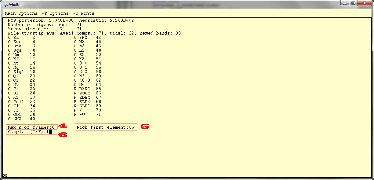
Figure 2 - Now the user has requested six frames and parameter 66
(which is the Polar motion amplitude) to be shown in the first
frame. The system will select the parameter with the highest
correlation as the other parameter. The confidence ellipse will be
shown with #66 ("POLM") on the abscissa and the other (#2, the
imaginary part of the annual tide, as it happens, labelled "Sa i",
on the ordinate.
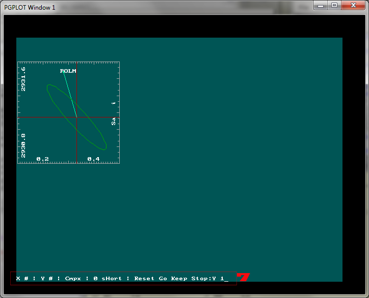
Figure 3 - The first frame has been drawn. The light-green bar
represents correlation, the length being scaled to half of the size
of the frame if it is 100%. The angle is derived from the
eigenvectors of the ellipse, (1/2) atan(v12/(v11-v22)).
The ellipse itself
is drawn on covariance axes. Thus, the permissible range of values
for the POLM amplitude can be read from the abscissa.
Since the analysis concerned gravity tides, the tide amplitude
computed by urtapt is *not* the delta factor but rather a ratio of
gravity [nm/s2] per equilibrium-tide elevation [m]. You
need to compare the ".prl"-result sheet and the ".trs"-table to find
out the ratio. A gravity option for grdcvem would be desirable. At
"7" the user selects parameter 1, the real part of the
solar annual tide, for the ordinate of frame 2. After entering "Y
1", the command that activates plotting is "g" (for Go).
The parameter for the X-axis is unchanged.
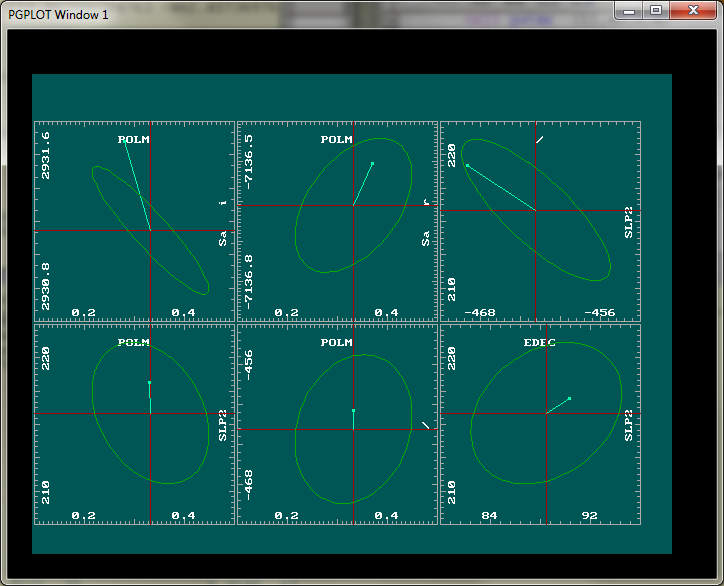
Figure 4 - Selecting five additional pairs after studying the
correlation file (sort -nr -k3 tt/urtap.pcorr) the screen is filled.
EDEC designates the second exponential that was excited due to the
repair in February 2011. A pair that shows high
correlation consists of the two slopes, the initial drift (symbol
"/") and the additional drift starting on February 24, 2011
(symbol SLP2). SLP2 consists of two parts, which are not
distinguished by symbol, only by parameter number.
An improvement here would add a sign to clarify whether it's the
bias or the slope part of the Box-car&Slope signal
(introduced in urtapt by Wavegroup command %) that is shown (perhaps
lower-case letters for the slope part).
.bye