USAGE:
hms-plot [options] YYMMDD HH:MM:SS duration-expr
PURPOSE:
Plot a segment of SCG data with HH:MM annotation.
First try to find data in d/...ts
If not found or insufficient duration, create the data
using tsf2ts-decim
YYMMDD
HH:MM:SS - start
date and time.
duration-expression - (no blanks!)
dh=hours or dm=minutes or ds=seconds
"dh=hours dm=minutes"
etc. is possible, e.g. "dh=1 dm=30".
OPTIONS:
FILES AND DATA
-f
ft
- ft = file
type
[A2]
-i
ind - ind = input
directory
[RAW_o054]
-d
r
- r =
sampling rate as part of file
name
[1s]
-c
c,c.. - c = channel
numbers
[none]
-n
n,n.. - n = channel
names
[none]
-u [u|c][[u|c]..
convert units (u), default is c,
straight [ccc...]
Volts. Position of symbol in string equals
channel number. u stands for (SI-) units,
c
for channel (historic) (!)
Example:
-u cuuuc -c 9,13,14,21,41
(disclaimer, GWR isn't consequent).
-e
e:e.. - e = tsf edit options, either
-- (dummy) or
a string
`file.tse,TRG´
[--:--:...]
-e
f - f = the name of a file with
lines containing
`-Efile.tse,TRG´ or in the order of
the channels.
OPTIONS:
PLOTTING
-N
- Prepare data, but do not plot.
-C
c,c.. - c = color codes (triplets) or
color names [bla,red,blu]
Names: bla blu red yel pur cya
tur
Additional colours must be defined in this
script; look for '# COLOR NAMES' .
If less colours are given than channels,
different grays will be used for the tail.
-Y
y,y.. - y = curve
offsets
[0,0...]
-S
s,s.. - s =
multipliers
[1,1...]
-D
b,b.. - b = 1 to remove DC-level, 0
to
retain
[1,1...]
-YR
ylo/yhi Overrides the
AUTO-detected Y-axis limits
-YT
t
t = tick interval,
overrides the AUTO-devsied one.
-LW
w
- w = legend
box
width
[1.2]
-LP
x/y - legend position, 0
< x < 8, 0 < y <
1
[7.9/0.01]
`'x-$legw/y-$legh'´
is possible.
Obs the framed box has a 10% outer margin along each edge
-PNG
d - convert
to png ( command = ps2png -rr -m -d d )
- d =
density or `+´ for
default 144x144
FILES:
./hmsticktable.awk
- given a sampling interval and a duration,
returns parameters for JDC to create a loop.
HOW TO ADD
CURVES:
(It needs care to get
the time right)
setenv
HMSADDCURVE file
where file is a csh source. Example
file: ./seismogram4hmsplot
which is a tslist
| ... | psxy pipeline plus an
set yloc = `echo
legend-text | addlegend $yloc ... command
HOW TO
PROCEED WITH BAROMETER DATA:
Prepare a file d/G1_3_$yymmdd-1s.ts
Rename the file so that
it fits the A2 or A1 type and devise
a channel number beyond
those of the A2 or A1, e.g. 77
Exec this script and
expect that a channel name is asked for.
There is an option
-xl
[d=delimiter] 'name,name...'
default delimiter = ,
so the name prompting is
bypassed. Specify the names in the
order of beyond-regular
channels.
EXAMPLE:
hms-plot
-c 9,21,41,77,78 -xl d=: 'Baro_[hPa]:Temp_[@+o@+C]' 120104
00:00:00 dh=48
EXAMPLE:
hms-plot -C red,tur -Y 0,0.5 -S 5,1
-c 9,10 120104 12:00:00 dh=1
-c 2 channels, 9 and 10
(alt: -n channels by names)
-C colours
-S scales
-Y offsets
120104 =
date 2012-01-04
12:00:00 = start time
dh=1
= 1h duration ( alt: dm=value in minutes, ds=value in
seconds)
You might have to update
~/bin/hmsticktable.awk
The following example is from this command set:
The result first:
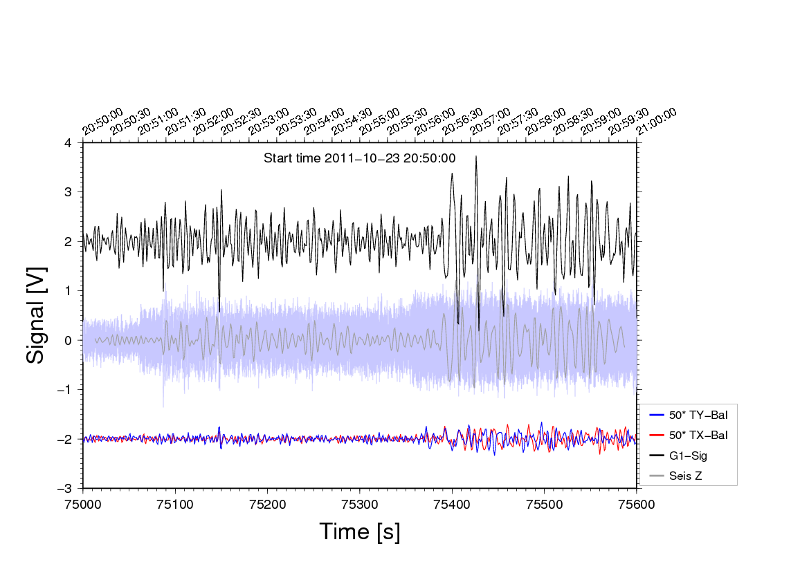
setenv
HMSADDCURVE seismogram4hmsplot
hms-plot -c
5,12,20 -o hms-5-12-20-treq.ps -LP '8.03/0.03' -S 1,50,50 -Y
2,-2,-2 111023 20:50:00 dm=10
Explanation:
-c Channels for
Gravity and Tilt balance
-LP legend position outside
the diagram space
-S scale tilts up
with factor 50
-Y move gravity up and
tilt down by 2V
dm=10 for 10 min duration
The source script:
#
Earthquake Turkey 2011 10 23 20:54
set eqd
= ( 2011 10 23 20 50 00 )
set
eqdur=60000
set
eqdoy = `cal2doy +d. +f%03.3i $eqd`
set
eqdoyc = `cal2doy +d: +f%03.3i $eqd`
set
eqdatt = `echo $eqd | awk '{gsub(/ /,",",$0);print $0}'`
set rm
= `calc -f "%02i" "int($eqd[5]/10)*10"`
echo
"tslist
~/Seismo/gcf/G${eqdoy}/GCF.${eqdoyc}:${eqd[4]}:${rm}:00.3U93Z2.ts
\
-BHc$eqdatt -Un$eqdur -Ediff.tse,DYDT -I \
-o ~/Seismo/gcf/G${eqdoy}/tmp.ts"
tslist
~/Seismo/gcf/G${eqdoy}/GCF.${eqdoyc}:${eqd[4]}:${rm}:00.3U93Z2.ts
\
-BHc$eqdatt -Un$eqdur -Ediff.tse,DYDT -I \
-o ~/Seismo/gcf/G${eqdoy}/tmp.ts
set
juld = `JDC -d -m $eqd`
set
juls = `JDC -d -m -S$juld -k2 $eqd`
set
secs = `calc "86400*$juls"`
echo
"tslist ~/Seismo/gcf/G${eqdoy}/tmp.ts -qqq -N -ns+$secs -D
-S0.0025"
tslist
~/Seismo/gcf/G${eqdoy}/tmp.ts -qqq -N -ns+$secs -D -S0.0025 |\
fgrep
-v '<' | psxy -R -JX -m -W3/200/200/255 -K -O >> $psout
#
low-pass filtered and decimated *100, filter length 2 * 600
samples ##################
#
#
set secs = `calc $secs+12`
tslist ~/Seismo/gcf/G${eqdoy}/tmp.ts -qqq -N -ns+$secs -D -S0.02
-Elpf.tse,LPF600 |\
fgrep -v '<' | psxy -R -JX -m -W3/160 -K -O >>
$psout
#
#
# End
low-pass filtered data
###########################################################
set
yloc=`echo "Seis Z" | sed 's/_/ /' | addlegend -y$yloc -d1
-W8/160`
Notice that the script is quite general; define date, time and
duration in the first two lines, and off you go.
The special part in it is the plotting of the low-pass filtered
seismogram. We skip a legend entry for the unfiltered data.