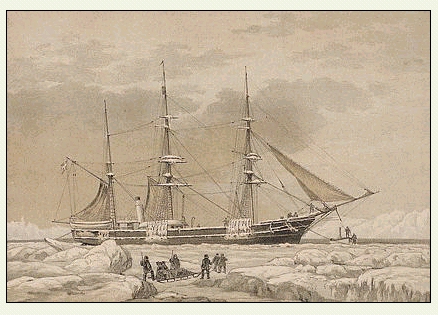
 Fig.1Fig.1
Instead of an introduction we show the measurements. They speak for
themselves.
 Fig.3
Fig.3
The measurement technique and some data analysis carried out at the
time are described in Rosén (1887). The series acquired while
Vega was immobilised due to sea ice is nearly flawless in coverage. Its
value and usefulness as a mareographic measurement is the subject of this
study.
To illustrate the efficiency of the observation effort we show the
whole series (bottom frame in Fig. 3) and, in order to discern individual
samples, a blow-up of the month of April (top frame).
Measuring water depth from onboard Vega.
The tide gauge measurements were made with cable that was anchored
at the sea bottom with cast-iron pigs. The cable ran into the Vega
hull via a tube and over a wheel that had been firmly attached to a Vega
deck. At the free end of the cable an iron cannonball served as a counterweight.
A pointer was attached to the cable pointing on a scale that had been graded
in units of "lines".
Corrections have been applied by the Vega crew to compensate for the varying water line of the floating vessel. During some periods these measuments were less certain for reasons of thick ice or greater than anticipated immersion.
Timing.
We have assumed that the Nordenskiöld expedition timed their measurements
from local solar time determinations. Local solar time was still a viable
concept in the 19'th century in Sweden, even railway stations along the
same line had their own time. The crew may also have used
their ship chronometre; in that case, the time scale of their place
of departure (Tromsö, Norway) may have been used. Our assumption
might be debated as there might be some doubt as to the notion of time
reference in Rosén's tidal data record. The most convincing clue
to us was the demarkation of the day and half-day boundaries that were
termed midnight and midday, respectively, which suggests a local relation.
Further, some time series analysis was carried out by Rosén (1887)
with a stacking method, using a basic solar day window length for
the determination of solar amplitiudes and phases, and equivalently one
with the length of a lunar day in the case of lunar tides. When Rosén
relates to a time lag of the tide he frequently uses the expressions for
solar or lunar transits. Also in conjunction with these operations, the
text appears to speak rather of local relations than of such which would
hold at the zero meridian. Greenwich meridian or zero meridian are not
expressly referred to in the text.
Turning to more recent standards, local mean solar time
at Pitlekaj is related to UTC by UTC + 12h27m28s
= UTC + 12.44107h = UTC + 44788s
In order to obtain a time equivalent to UTC but for 1879, one
can subtract 0.77 leap seconds per year. A semidiurnal tide advances in
90s by 0.77o, which is relatively small. A one meter high tide
changes by as much as 0.013 m during 90s. Thus, an accurate account of
the deceleration of earth rotation is not critical at the order of seconds
for tidal analysis of data with an SNR of 100:1 or less.
Pitlekaj is situated near Bering sound at longitude W173o
23' 02", latitude N67o 04' 49". Thus, there might be a question
as to the date.
Note that the longitude is West of Greenwich, but according to international
conventions the Datum Border has not been passed.
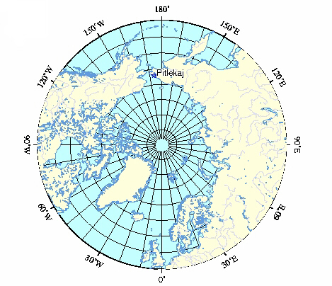 Fig. 4
Tide analysis.
The model for the tide generating forces that was employed for this
study is the one by Tamura (1987). It contains roughly 1200 different
tide waves and covers spherical harmonics to degree and order four. Response
parameters where estimated that each relate a group of model waves
to the local observations. The division into groups is based on the frequency
resolution capability, which is primarily dependent on the duration
of the measurements. Half a year of measurements, for instance, is suffiecient
to fully discriminate between the lunar and the solar declinational waves
called K1 and P1 (their beat period is 0.5 tropical years). Below, the
wavegroups will be represented by their most prominent members (central
to the frequency band, large in magnitude), and the frequency will be given
along with the Darwin symbol (K1 etc.).
The parameter estimation method uses a least-squares procedure. Since the premise of least-squares in this case is to determine sinusoidal wave packets in white noise (emphasis on white noise), the time-series must be preconditioned in order to meet this criterion. In many cases of naturally occurring processes, long-term periodic or aperiodic variations are encountered. An efficient way to obtain white noise from a coloured noise process is by means of the Maximum Entropy method. From this one obtains a prediction error filter which is to be applied an both the time-series and the model wave groups. Such filters designed for air pressure, water level or similar processes have typically five to ten coefficients, and their effect is to decorrelate subsequent data points. Deterministic filters like the familiar Butterworth or Chebychev designs may yield a sharp suppression of unwanted signal components; however, their effect on the stochastic properties of time-series is rather to distribute additional correlation between many samples even far apart from each other.
The particular least-squares solution method that is used here goes under the name of Generalized Inverse or Lanczos Inverse (Aki and Richards, 1980); it has a near relationship to Singular Value Decomposition. The advantage is that such methods are robust in situations of accidental overparametrisation, like when model signals are virtually indistinguishable.
Tides in the Pitlekaj area according to modern tide
models.
The local coastline is reasonably complicated near Pitlekaj. In order
to resolve the basin geometry, a 1x1 degree mesh as in the case of the
Schwiderski (1980) tide atlas is not fine enough. Also the 0.5x0.5
degree mesh of Le Provost et al. (1994) has not the sufficient resolving
power to obtain continuity between the tide in the Pitlekaj bay and the
open Arctic. It is thus found that modern models do have problems in the
area in question, and that the Vega data might actually contribute valuable
data for constructing an improved, regional tide model. This, however,
would digress too far from the subject of this report.
In order to evaluate the Vega tide parameters for Pitlekaj we can still
employ a tide model like Le Provost et al. (1994) after giving reasonable
discount as to its average accuracy. Also, using the bay value
directly from the Le Provost model appears less convincing than looking
for comparison in the surrounding. Small bays that are connected to open
waters through a strait or a gatt often follow passively with the open
ocean tide just outside the mouth except in rare cases of large bays with
very low water depth. In the model, the bay might have been connected through
only a single node, which may introduce large local errors in the solution.
The following three figures are from the model of Le Provost et
al. (1994). We show the diurnal O1 tide and the semidiurnal M2 tide,
the latter also in a regional zoom-in. The resolution of the coastline
near Pitlekaj appears quite rough. In particular, the bay is represented
by a single model node that is diagonally connected to the northeast with
another semi-isolated note. Both amplitudes and phases appear highly discontinuous
when compared to the more open waters to the north.
 Fig. 5a-c
The letters A and B
in Fig. 5c indicate the M2 tide information near Pitlekaj obtained from
the Le Provost et al (1994) numerical model. The result from the analysis
of the Vega data for the M2 tide (3.0 cm, -8o) is
in bad agreement with the model tide at the node closest to Pitlekaj
(B) and also at the neighbour
node A , phases differing by
near 180 degrees. However, the model amplitudes at A
and beyond are at least a factor of two larger. Results for the S2
tide are similar: Model phases in the area are between 270o
and 180o, while the observed phase is 56o.
The O1 tide shows a phase discrepancy on the order of 180o,
too. A 180o phase change could result from a misinterpretation
of the mathematical sign of the records. My understanding has been that
the readings increase when the water level falls. Trying to explain the
problem , there could be a faulty epoch or faulty longitude specification
to the analysis program; however, the consequences of such misalignments
would be seen differently in the diurnal and semidiurnal, solar, and lunar
species, respectively.
Reasons for the attenuation in the ice-covered bay may be a fertile subject of speculation.
Table 2 shows some important tides, comparing two models (Schwiderski 1980, Le Provost et al., 1994) with the observations. Given that we mixed up a minus sign, the Schwiderski model is very close to the observed tides while Le Provost et al. in most cases predicts amplitudes a factor of two larger and significantly different in phase. The Mf tide results do not contradict this proposition regarding the large error parameter of this long-period tide.
To arrive at correct results we have therefore assumed a sign inversion, i.e. that the tabled values in Rosén (1887) specify water depth. The cophase column of Table 1 should be incremented by 180 degrees. The conversion has (not yet) been done in Figures 6 and 7.
Table 1. Results of tide analysis. The harmonic coefficients
of the Pitlekaj tides determined from the Vega data
are given in terms of amplitudes [m] and phase. The phase specifies
the lag angle [o] with respect to the corre-
sponding astronomical tide at Greenwich meridian. The 95% confidence
limit is derived a posterori assuming
a standard normal error distribution of the residual.
The analysis was carried out for an Earth with a liquid core.
The latter introduces a resonant term in the tide
generating potential at diurnal frequencies (blurred numbers).
Table 2. Comparison of tide models (L - Le Provost et al.
1994, S - Schwiderski (1980) with the observations at Pitlekaj. A 180 degree
phase shift may have arisen due to a misunderstanding in the specification
of the records, whether positive changes represent rising or falling sea
level.
The harmonic results can also be shown in the form of gain factors by dividing the ocean tide amplitudes by the amplitude of the tide potential. The result shows usually a slight frequency dependence across a tide band. The tide response of an ocean area can be discribed as a superposition of resonant modes, much like the resonant strings that a number of musical instruments possess (sitars, certain guitars and lutes, the famous swedish key harp, etc.). The excitation process in each case is a compound signal with a finite number of slightly distorted sinusoids, and the resonant strings or oceanic oscillatory systems contribute to the compound response in reciprocal proportion to the difference in frequency. The richer the resonant structure of the ocean area or the number of resonant strings, the richer of features is the gain spectrum. However, a detailed study of the gain spectrum requires a high signal-to-noise ratio of the measurements. The present data set is a bit limited in this aspect. We show the gain spectrum below, first showing results from almost all tide bands that had been set up, then only the stastically significant results on a 95 percent confidence level. In the former case, the error circles are partly very large, so we have scaled the errors in Fig.6 down by a factor of 100.
Although generally small---at the level of only a couple of centimeters---the most important semidiurnal tides (N2 M2 S2 K2) are well determined. The diurnal tides appear smaller still. In that frequency band, only three wave groups showed up above the noise level: O1 P1 and K1.
Results for the long-period tide Ssa (semi-annual) are highly
uncertain as the signal duration is only slightly greater than 0.5 yr,
and long-periodic noise was a strongly present. Thus, these results were
suppressed. The annual tide (Sa) was not included in the model
since the duration of the data is much less than one year. The monthly
and fortnightly tides (Mm, Mf) are found to have
insignificant amplitudes with respect to a 95% level of confidence, much
owing to the higher noise level at these low frequencies.
Fig. 6 Gain spectrum. Each frame shows a fundamental
frequency band. The gain is represented as a so-
called phasor arrow. The foot of each arrow is placed at the frequency
of the tide, read from the horizontal
axis. The length of the arrow represents the efficiency of the response
(compare with scale along the
vertical axis), and the direction represents the phase lag with
respect to the corresponding astronomical
tide at the Greenwich meridian. For this figure, the error limits
(the circles centred on the arrow heads)
have been scaled down by 0.01.
Fig. 7 Gain spectrum of significant tide wave groups. Here,
the error circles are drawn to
scale and represent 95 percent confidence limits.
Looking at the residual.
After the least-squares fit of the tidal model the postfit residual
appears to be mostly white-noise, i.e. fulfill the normal error criterion.
The variance parameter for the least-squares has been taken from the RMS
of the series shown here below as a kind of hindsight justification in
lieu of a priori information about the measurement error. If one considers
the variable sea level as part of the noise of the measurement process,
then only the hindsight variance is objectively available; the reading
error of the scale would probably be an overoptimistic guess.
Fig. 8 Filtered residual time-series.
Power spectrum analysis of the residual.
In order to judge the efficiency of the least-squares fit, the residual
is analysed with standard time-series analysis
techniques (e.g. Oppenheim and Schafer, 1975).
Power spectrum analysis shows that the residual is a little
overwhitened, and that there is residual semidiurnal spectral power. The
reason for that is most often that there are temporary perturbations, like
solar synchronous thermal tides that affect the measurements only during
days with clear skies, or time-varying calibration of the measurement
device. There might be other reasons. The overwhitening, i.e. the exaggerating
action of the prediction error filter, is a direct consequence of these
nonstationary signal components.
Fig. 9 Power spectrum of filtered residual The
objective of the filter is to obtain white noise.
Acknowledgment.
The records of the Rosén paper have kindly been transferred
to computer
readable form by Britt-Marie. Graphic procedures have been provided
by
Wessel and Smith (1995).
References.
Aki, K. and Richards, P. G., 1980. Quantitative Seismology, Theory
and Methods, Volume II, Freeman, San Francisco,
pp. 559--935.
Le Provost, C., Genco, M. L., Lyard, F., Vincent, P., and Canceil,
P.,
1994: Spectroscopy of the world ocean tides from a finite
element
hydrological model, J. Geophys. Res., 99,
24777--24798.
Oppenheim, A.V.,and Schafer, R.W, 1975. Digital Signal Processing,
Prentice Hall, Englewood Cliffs, 585pp.
Rosén, P.G., 1887. Iakttagelser av Tidvattnet vid Pitlekaj under
Vega-
Expeditionen 1878-79, ur Vega-expeditionens vetenskapliga
iakttagelser, Kungliga Vetenskapsakademien ? Stockholm.
Schwiderski, E.W., 1980. On charting global ocean tides, Rev.
Geophys. Space Phys., 18, 243-268, 1980
Tamura, Y., 1987, A harmonic development of the tide-generating
potential, Bull. d'Inform. Marées
Terr., 99, pp. 6813--6855.
Wessel, P. and Smith, W.H.F., 1995. New version of the Generic Mapping
Tools released, EOS Trans. American Geophys. Union,
76, p329.
Illustrations.: Fig. 1,2 - Nationalencyclopedien, Bra
Böcker, Höganäs. Demo-CD. Fig. 3,...
- produced with GMT (Wessel and Smith, 1995).