Ocean tide loading

The earth surface dips under the load of the ocean tide. This phenomenon is greatest under the load, i.e. on the continental shelves, but it also extends inland. A simple way to characterise the phenomenon is to

(1) split the tides up into a harmonic spectrum of discrete periods. For instance the semi-diurnal lunar wave and the semi-diurnal solar wave are quite well known. Their periods are such that every 14 days the two effects add to each other, or if you like, every 14 days they subtract from each other, leading to the famous spring and neap tides, one week apart. Less well known is the fact that we have diurnal tides, which depened on the position of moon and sun above the equatorial plane. Thus, they completely vanish two times per month. With four diurnal and four semidiurnal waves we can represent most of the time dependence of the ocean tide, und thus also of its consequences, e.g. the loading tides.

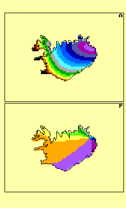
(2) for every such wave to compute the amount of dip at the earth surface, and the time lag with respect to the maximum gravity tide at Greenwich meridian. These two quantities are Amplitude and Phase of the loading tide. Consider the Iceland example below. At Reykjavik the amplitude of the principal lunar effect (M2) is 15 mm and the phase 350 degrees. 360 degrees means one full cycle or 12.4206 hours, thus Reykavik is most "up" 0.345 hours before London experiences the strongest gravity pull. For this one wave (but it's the most important one in the North Atlantic).

These effects can be quite large. In Brittany, in Cornwall, and also at the "knee" of Brazil, the vertical displacement can amount to 0.1 m. Needless to say that this motion must be quantified when we conduct geodetic measurements aiming at the millimetre level.

What is a little more difficult to accept is that the earth crust also moves horizontally. This movements are largely coordinated with the vertical motion. Basically, the displacement is towards a subsiding and away from a rising area. It's a bit less clear if you are in areas where the vertical displacement has saddles or is flat. In space geodesy we need to know all components of the motion in the three dimensions).

For more information please refer to our Automatic Ocean Tide Loading Service

Ocean Loading Example:

Radial displacement due to M2 tide in Icelandic sea.

Using LeProvost tide.	Using Schwiderski tide.

Top frame shows amplitude in metres.

Bottom frame shows phase relative astronomical argument at Greenwich (expression is cos(arg - pha)) in degrees.

Software

A. Programs for tide time series computation.

A.a Interpolating the admittance spectrum linearly.

There is a simple main program to compute Radial, East and North displacements (name ttism.f.) Click here to get the code in unix tar, current version number is 109 (March 2000). There is also an instructive little main program ttifm.f that demonstrates how you can cut down the time and space burden. The tar contains also a perhaps unnecessarily complicated program named ttimm. It shows what you can do with the accompanying library routines.

Read more about it.

A.b Interpolating the admittance spectrum with orthotides.
A new, simple procedure to compute time series of loading tides is available. You typically launch it from a command line

   oltidem -h

# prints a short help text

   oltidem -F $MYFTP/oload/olls27.blq -L 11.9,57.4 -X -D 1998,2,25 -O test.prt

To adapt it to your needs you must plough reading through p/m/oltidem.f and p/oltidets.f. The unix tar-file is here. You can read more about it.

See the IERS Conventions 2000, Chapter 7

B. Programs for ocean loading computation, the global stage.

B.a Program to do the loading computations on a per-site basis.
The program's name is olfg. Click here to get the code in unix tar form.

Read more about olfg. Program documentation (very technical) is available here. The following link may be more actual. There is a simple online-manual too.

B.b Program to interpolate on gridded ocean loading effects.
We have global maps of ocean loading tides (radial displacements and vector potential of tangential displacement). Resolution is 0.5^o x 0.5^o. The ASCII files require 36+ Mbyte space. The associated program to interpolate on these grids is called olmg. It is available here. For space reasons we cannot offer the maps online. If you decide that olmg is your choice, create an incoming area on your ftp server and send an e-mail; the files will be copied to your site.

C. Post-Processor for olfg

The program's name is olmpp. Click here to get the code in unix tar form. A users's guide is included in the tar and available here.

You will need pgplot for X-Windows interactive screen graphics.

A global topographic database is required. Since olmpp has been written in FORTRAN, the topo data must be reformatted to fit the binary file blocking convention. Recommended: ETOPO5 or TerrainBase from the National Geophysical Data Center, NOAA You may need to reformat that data base for Fortran binary read access. Here is a basic program that shows the essentials.