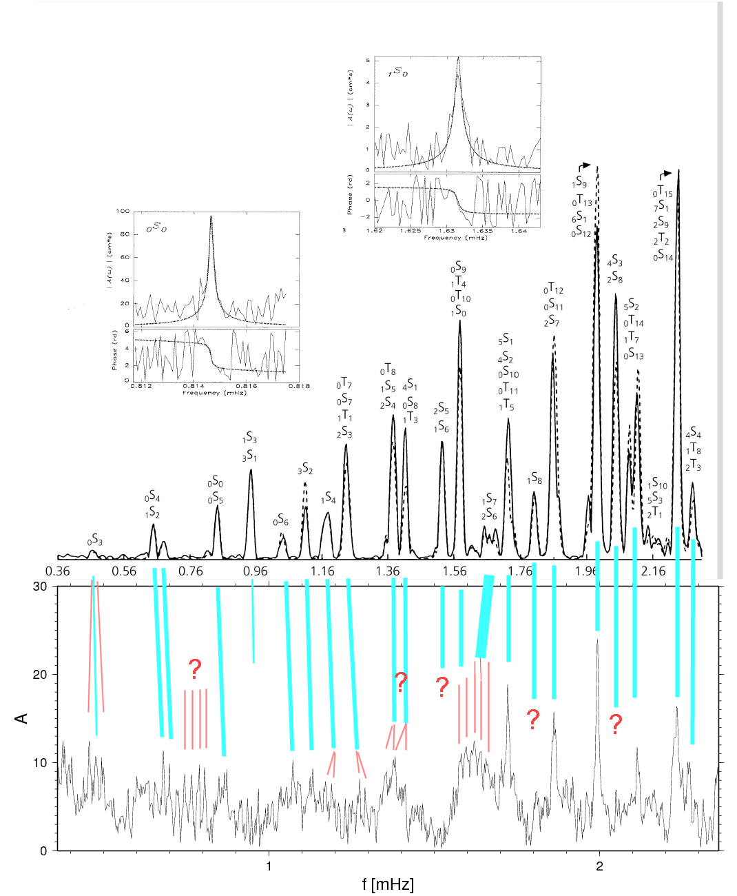
News from GWR 054, the Superconducting Gravimeter at Onsala Space Observatory

 - Earthquakes and Free Oscillations


2010 Mar. 08

After the Magnitude 8.8 - Earthquake offshore Maule, Chile, 2010-Feb-27 at 06:34:14 UTC


Above figure (click to enlarge) shows the free-oscillation spectrum obtained from 15 days of SCG gravity after the M8.8 earthquake offshore Maule, Chile, on Feb. 27, 2010 at 06:34:14 UTC (barometric effects reduced). Some of the low-frequency modes have been marked. Klick into the image to see it in original size. Note the splitting of the lines of the 0S3 and 0S4 modes, a consequence of the Coriolis effect. Earthquakes closer to the equator would show even greater splitting. In the Padang example below you will see a triplet for 0S3.
Also note that the sharp line next to 0S5   the "breathing mode" 0S0 at 0.817 mHz.
The lowest known eigenmode of the earth, where the deformation resembles the shape of an American football, labelled 0S2 has also been observed; its period is 54 minutes. Known means here "confirmed by observation". A search for an inner-outer core oscillation, the so-called Slichter mode (4-8 hours period), is still under way. The Global Geodynamics Project (GGP) is working on the problem. Maybe the 2010 Chile earthquake has finally lifted the oscillation above the noise floor. The big one in Chile in 1960 didn't although it had a magnitude of 9.6 but instrumentation has improved since then, and GGP is coordinating a world-wide network today. See also Duo et al (2007) .

The mode symbols are to be interpreted as follows:
S or T designate spheroidal or torsional deformation, respectively. Spheriodal modes are curl-free, and contain a sizable fraction of motion in the vertical. Thus, a gravimeter is a sensible instrument for their measurement. Toroidal modes would have no vertical component if the earth would not spin. However, the small accelerations that a mass particle experiences as it moves at right angle to the rotation vector produces a force that in general also has a vertical component (i.e. radially from the earth centre). This is commonly known as a Coriolis-effect.

The subscript to the right of the T or S mode symbol expresses how many node lines there are encircling the earth, either parallel to each other or crossing at right-angle. This is like an oscillating membrane draped over a sphere. In each node line, deformation is zero; across the node line, deformation reverses its sign.

The subsript to the left of the symbol expreses how many node surfaces there are in the interior of the earth. Again, deformation is zero on these surfaces. They are concentric like in an onion.


See Virtanen (2006) for more details on the subject matter.

The breathing mode can be followed for a long time (more than the 59 days of the following plot)

Watch the signal power at 0.817 mHz slowly decaying. The black band is due to an earthquake on April 4, 2010 (Baja California, Mw=7.2).

Surface displacements

We have double-integrated a band-pass filtered 1-s time series in order to obtain an impression of the size of the surface-wave displacement at Onsala:

A sign of first motion is found at  6:50 UT. The biggest surface waves arrive around 7:30 UT. Almost all peaks brought the gravimeter's ADC into saturation. We had to resort to a (admitted: home-grown) signal restoration technique
Visit the Displacements from surface waves news page !


After the earthquakes of Samoa and Padang/Sumatra Sep 29-30.

We show four images.Click on the blue-framed diagrams (Fig. 1 and 2) to obtain larger-scale figures.

Figure 1  - Sliding-window RMS (a kind of UV-meter like the one on your audio amp at home) showing how the coda of the Samoa earthquake is intercepted by the strike at Padang. Both events caused free-oscillations, the "ringing bell of the earth". The mode channel was used (a bandpass filtered acceleration signal) at 1 min sampling rate.


Figure 2 - Periodogram from a mode-channel data segment starting Sep 30, 13:00 UT and ending Oct. 4 (incl), i.e. including only the Sumatra event.
Possible improvements for this figure: Reduction for air pressure. (Don't think there's much to be gained though)


Figure 3: An attempt to identify low-frequency normal-modes. The frame in the bottom is the lower part of the spectrum of Fig. 2. The upper part is a spectrum from the earthquake of Bolivia, June 9, 1994. The two zoom-ups of 0S0 and 1S0 are from E.A. Okal, GRL 23:5, 431-434, 1996. The question is, whether the mode splitting indicated by the read lines is realistic. Observe that the gravimeter is largely insensitive to the toroidal modes (sTn).


Figure 4 - Short-time Fourier transforms of the 1-s acceleration data (1024 samples per batch, the window been shifted 256 samples). The amplitude scale (colors according to the legend on top) is logarithmic. On those particular days the microseismic level was a bit high (the orange band between 5 and 6 Hz) - you can see that it wanes towards the end of Sep.30.