Displacements at Onsala inferred from the Superconducting
Gravimeter for the Maule Earthquake of 2010-02-27
Summary
The first two figures show the surface wave displacements inferred
from the gravimeter record of the morning of Feb. 27, 2010.
The analysis suggests: 4 mm peak-to-peak
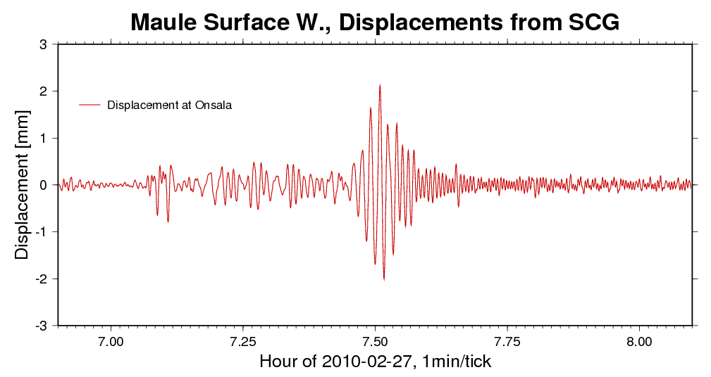
Figure 1 - Resulting
displacements derived according to the description on this page.
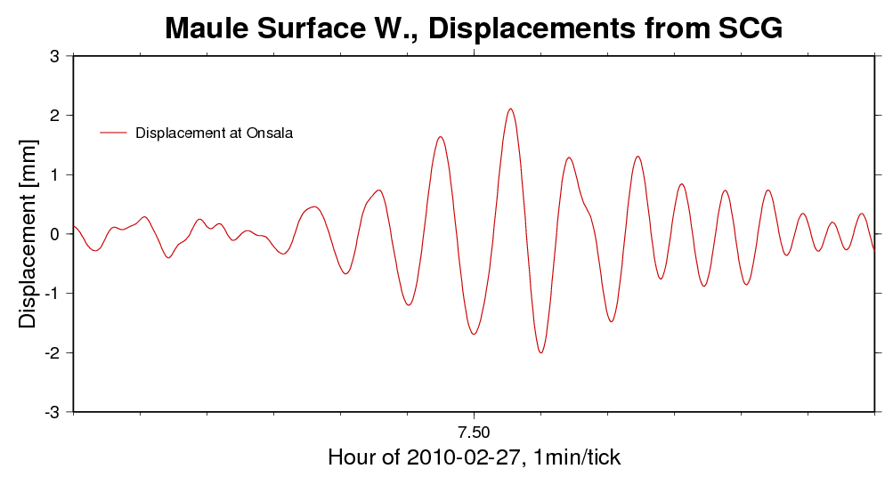
Figure 2 - Zooming on the maximum surface wave action ±6 minutes
around 07:30:00 UT.
Deriving these charts was no simple task. The SCG record clips at
±10 V (0.776 mGal), and the accelerations were much larger
thant this during much of the surface wave action. Figure 3 shows the
clipped and the restored signals. See "Signal
restoration" below; the process will be
desginated with symbol CSR for
clipped signal restoration.
In principle, displacements can be computed by double-integration over
time with carefully constraining the constants of integration. In the
present case, the signal was high-pass filtered (HPF) (suppressing a narrow range
near zero frequency (0 - 10 mHz) and a sharp transition to the
pass-band (121 + 121 filter coefficients using a Kaiser-Bessel Window
design with shape parameter 2.1. Spurious DC-offsets were deleted (DCD).
Integration was carried out with the simple scheme
INT: y(i+1) = y(i) + x(i) dt
which advances series y by 1/2 time
step, dt = 1s
u = DCD ( HPF ( INT ( DCD ( INT ( HPF ( DCD ( CSR (
DCD ( x
)))))))))
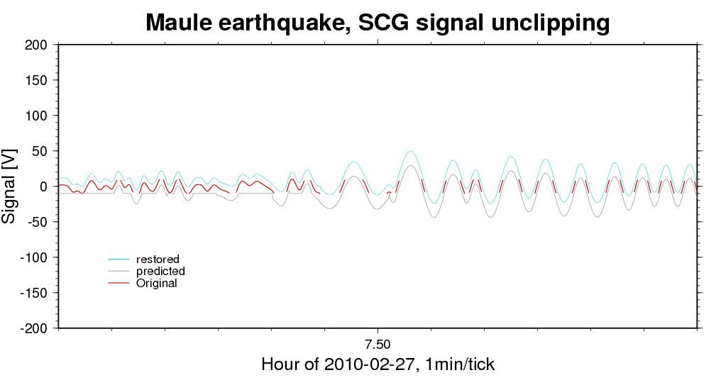
Figure 3 - Signal restoration.
The original gravimeter data with over-range values deleted (red
curve), and the restored signal (in cyan).
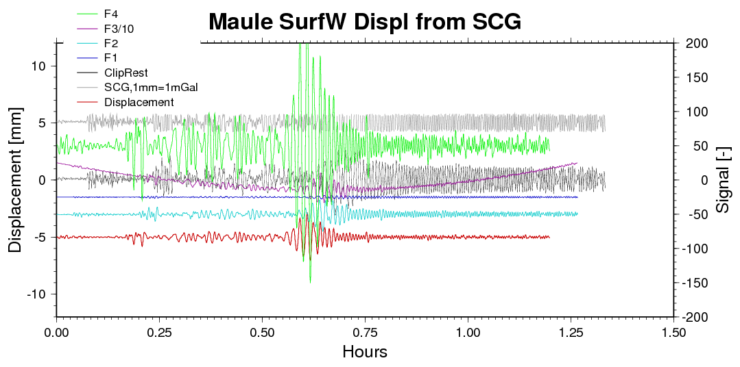
Figure 4 - Stages of signal
restoration and displacement computation. The time series are not
synchronous; SCG and ClipRest are unaffected by the 121-s truncation of
the high-pass filter, and F4 and Displacement are affected two times by
the truncation. F1 (dark blue) is after the first hi-pass, F2 (petrol)
after the first integration, F3 (purple) after the second
integration, and F4 (green) afterthe second filtering.
Signal
restoration.
This might be a matter of debate. The method employed was to
(1) cut the signal at ±10V and identify the gaps
(2) before and after each gap, find the times where maximum signal
change (x(i+1) - x(i))
occurs.
(3) a sinus half-wave is clamped with its zero-crossings at these two
points, from which we get the frequency
(4) a linear ramp is added to run through these two points.
(5) the sine is given a linearly changing amplitude since the slope in
the branches before and after the breaks may not be mirror-symmetric.
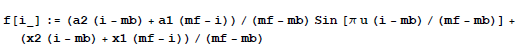
So there are four parameters to solve for the interpolation formula:
Sine amplitude: a1 and a2; ramp start and end ordinate: x1 and x2. The clamping points before and
after the gap are named mb
and mf (m-backward,
m-forward), respectively.
See the Mathematica notebook
print-out (pdf).
The fit is done with a nonlinear minimum finder (Numerical Recipes
dfpmin); the reason for this is that we anticipated (erroneously) that
we could adjust the frequency. All too often, the frequency parameter
runs away, so that many more than half a cycle is filled into the gap.
You may ask for the routines unclip.f (F77) and ask the
author of this page for Ddfpmin.f Dlnsrch.f (Num.Recipes slightly
adapted for the present purpose).
The procedure which carried out the process is tslist
/ tsfedit
(=> UNCLIP) (=> IIR) (=> FILTER D:WD), see the resulting
protocol of the process.
The relations of gravity to displacement are more complicated when
periods are long (mHz or below) - see a pdf memo.
Göteborg, 2010-07-12
Hans-Georg Scherneck
.