Maxwell root finding

Hans-Georg Scherneck, July 2013

All figures: Right-click and open in new window if you like.

§1 - Mode iteration and root finding in maxwell.f

We have a closer look at the free viscous modes for the model l96 um0.5 lm10. Figure 1 shows the modes detected using the control block
2 200 1
: -6 -1 0.0001      1.d-12
: -1  0 0.00002     1.d-8
   0  1 0.00005     1.d-8
500 12 1.5d0

See remark 1
The mode discrepancy is shown with small square symbols and dark draping below. You notice that there are outliers where the discrepancy goes up to order of 1. In the next paragraph we take a closer look at two cases, n=90 (big discrepancy, 0.707) and n=91 (normal, 0.011).


Remark 1
For dismissing small-strength modes the criterion was
   Mj / sj < Mcrit
where Mcrit is specified in the fourth column of the control block.

It was found that the diff.-eq. propagator at s < 10-5 produced unstable and big values for the secular determinant, order of magnitude exceeding 10100. These modes would be important only on the 100 Myr time scale, so subsequently the root search was started from √10 ×10-5/kyr

Figure 1 - Modes' Laplace-s versus spherical harmonic degree for radial displacement. Mode strength is indicated by symbols, see legend. Note the outliers of the asymptotic closure, mode sum at infinite time minus the "fluid" Love number.


§2 - Calm waters

In Figure 2 the slower modes for n=90 and n=91 are shown. The target parameter is the secular determinant (SD).

Figure 2 - Modes between √10 ×10-5/kyr and 0.1/kyr for degree 90 and 91. The logarithm of the absolute value of the SD is shown. Red or yellow curve sections correspond to positive, blue and cyan to negative values of the SD.  The zero-crossings that are accepted as free modes are numbered.
   The slow branch to the left has no obvious zero-crossing tendency until heavy (numeric?) noise sets in below 10-5/kyr (sign changes appear to happen randomly).

§3 - Difficult subdomains for Laplace-s

In the range between 0.1 to 10 /kyr a number of complicated looking features appear, see Figure 3a. From the left to the right:
  1. At log(s) ∼ -0.5 but below -0.45 is a band of wide scatter. It is bounded to the low end by a pole.
  2. Between -0.45 and -0.3 is a band of narrow scatter and an embedded zero crossing.
  3. Repeated poles and zero-crossings up to 0.
  4. A smooth segment with two zero-crossings between 0 and 0.3
  5. (different again!?)
Whether the complicated looking high end has similar features to 1. or 2. needs further investigation at this time. We can take a closer look at the range between -0.4 and -0.3 in Figure 3b.

Figure 3a - Like Fig.2, for n=91 however. Modes that are accepted using a tolerant criterion for slope convergence in the root iteration are marked by crosses.

Figure 3b - note the modes with number 63 and 69. The latter is at the zero-crossing (blue-to-red), whereas the SD around the former stays at negative values (blue), except that there are a few spurious positive points in the vicinity. This is the cause of the root iteration that resulted in the acceptance of the mode #63

§4 - Iteration and the slope parameter

When the zero-crossing is iterated by bisection, a key parameter called slope is determined. It is the limit of (s+h)/(SD(s+h)-SD(s)) for h → 0. 

The spurious signatures in the band of s appear to be characterized by
  1. small SD-values of the opposite sign and
  2. a steepening slope as the iteration homes in on the zero.
Thus a criterion:
Given a narrow sampling of the s domain, the slope must not change more than 1 percent during iteration.

Figure 4 - Left: Iteration of the slope parameter in the alleged mode #63.  The tolerant criterion has already dismissed many zero-crossings, so zero-crossing number 107 is actually identical to mode number #63, and 117 to #69.
The ordinate values have been normalised to the range of the SD at the outer points of the interval.

§5 - With a tight slope criterion

With the tight criterion, slope to be constant within 1% throughout the iteration (12 bisections), none of the spurious cases is accepted as a proper mode any more (Figure 5a) while the 117'th zero-crossing is accepted as a mode. It has now #16. The criterion is insufficient though to resolve the complications in band 1 (§3). 

Figure 5a


Figure 5b

§5 cont'd

The following instruction block
: -6 -1 0.0001      1.d-12
: -1  0 0.00002     1.d-10       SLC
   0  1 0.00005     1.d-10       SLC
500 12 1.01d0
(see remark below)
now finds 56 roots and no pole is misidentified. Almost 1000 cases of sign-reversals are found. Observe that the scanning intervals are very small. In an attempt to broaden the steps by a factor of ten, half of the roots are missed, all of them in the two upper ranges [-1,0], [0,+1].

Thus, there seems no way of of the small steps and hence the burden of long computation time. Two to three minutes of wall-time on my 64bit linux. Here's a little time saver: Instead of computing both of the SD's bracket values, the previous value for the higher s is re-used for the lower s. And an instability in the slope parameter during iteration can be determined early and the loop be terminated.

Remark
New instruction SLC = apply slope convergence criterion
New parameter Q (e.g. 1.01d0):
1/Q < q < Q, where q = ratio of slopes, at start and end of iteration

Figure 5c - Inspected zero-crossings are numbered in the upper row, identified roots in the lower row of numbers; they belong to n=90. The SD for n=91 is only shown as a graph. 

§ 6 - Leg pullers

For the examples here (Figure 6) three kinds of counter-measures can be used:
1. smaller scanning steps;
2. a more tolerant SLC;
3. deeper iteration.

@3: I was using Nb = 12 bisections. The code for the criterion is such that the Nb'th slope is compared with the slopes of the bisection steps k from max[1, (Nb-11)] to Nb-1; the slope ratios would remain near unity
1/Q < qk < Q, Nb-12 < k < Nb
The code could be changed to make the 11 adaptive when there's hope, or just user-controlled.
After inspection of the solution for a range of sph. harm. degree, looking for outliers in the fluid discrepancy, only a limited number of degrees would require recomputing.


Figure 6 - Note the flip in structure near the centre for n=5, which does not occur for n=4. The zero-cross numbers (upper row) are #61 and #63. At #61 the root misses the slope convergence criterion 1.01 but would yield to 1.02 .
At #63 the miss is very near, 1.0103 would have caught the prey.


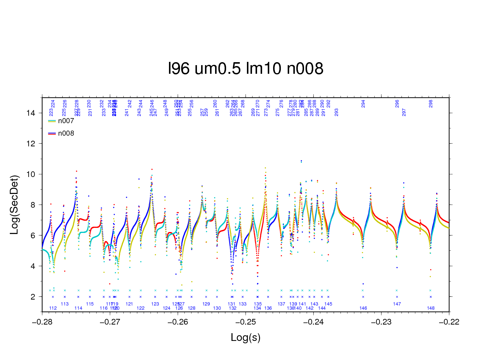
§7 - Resistant bummers

This case (n = 69, s = 0.4303, log s = -0.3662) can only be solved with a narrower base interval.
And a more tolerant slope convergence criterion. Two missed 
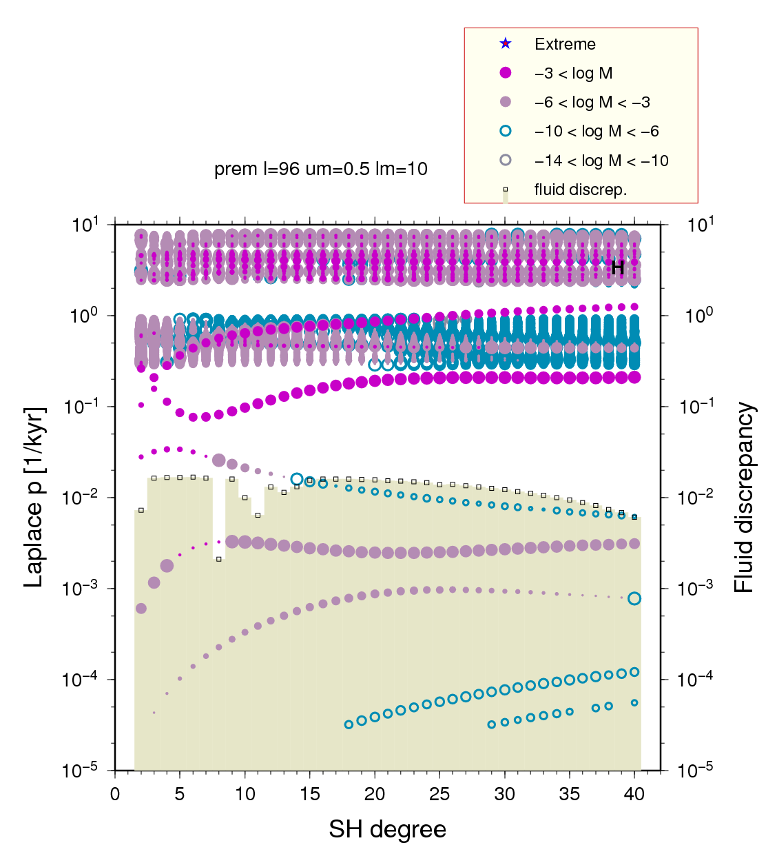
roots located within close range cause a significant outlier in the fluid-discrepancy test. The roots are important as their relaxation times are 2,300 yr.  At n=70 the world is in order again.

The slope series during the iteration is
Table 7a: Iteration of zero-crossing #120
-----------------------------------------------
 k       log(s)         slope     slope/slope12
-----------------------------------------------
 1 -3.66192500e-01  -3.12772e-42    0.954691
 2 -3.66193750e-01  -3.33959e-42    1.019361
 3 -3.66193125e-01  -3.46286e-42    1.056987
 4 -3.66192812e-01  -3.53379e-42    1.078638
 5 -3.66192656e-01  -3.52338e-42    1.075460
 6 -3.66192734e-01  -3.51812e-42    1.073855
 7 -3.66192773e-01  -3.49597e-42    1.067094
 8 -3.66192754e-01  -3.55244e-42    1.084330
 9 -3.66192744e-01  -3.37290e-42    1.029528
10 -3.66192749e-01  -3.28091e-42    1.001450
11 -3.66192751e-01  -4.22279e-42    1.288945
12 -3.66192753e-01  -3.27616e-42    1.000000
-----------------------------------------------
The eleventh value might suffer from imprecision.

It's even worse at zero-crossing #121:
Table 7a: Iteration of zero-crossing #121
-----------------------------------------------
 k       log(s)         slope     slope/slope12
-----------------------------------------------
 
1 -3.66182500e-01  2.48226e-42    2.137116

 2 -3.66181250e-01  2.15139e-42    1.852251
 3 -3.66180625e-01  2.31567e-42    1.993689
 4 -3.66180937e-01  2.41021e-42    2.075084
 5 -3.66181094e-01  2.48145e-42    2.136418
 6 -3.66181172e-01  2.44919e-42    2.108644
 7 -3.66181211e-01  2.36189e-42    2.033483
 8 -3.66181191e-01  2.44075e-42    2.101378
 9 -3.66181182e-01  2.72824e-42    2.348894
10 -3.66181177e-01  2.61868e-42    2.254567
11 -3.66181179e-01  1.33728e-42    1.151339
12 -3.66181178e-01  1.16150e-42    1.000000
-----------------------------------------------

A special scan of the problem laden s-range
 -0.368 -0.364  0.000005    1.d-10    SLC
500 12 5.0d0 4
determines the two roots and the associated Love number strengths as follows:
n,m          |        69     2
s            |  0.43033557E+00  0.43034704E+00
h,l,k elastic| -0.27471472E+01  0.84046976E+00  0.00000000E+00  0.00000000E+00 -0.14401682E+01
h,l,k asympt.| -0.16485111E+02  0.75387823E+01  0.00000000E+00  0.00000000E+00 -0.13183694E+02
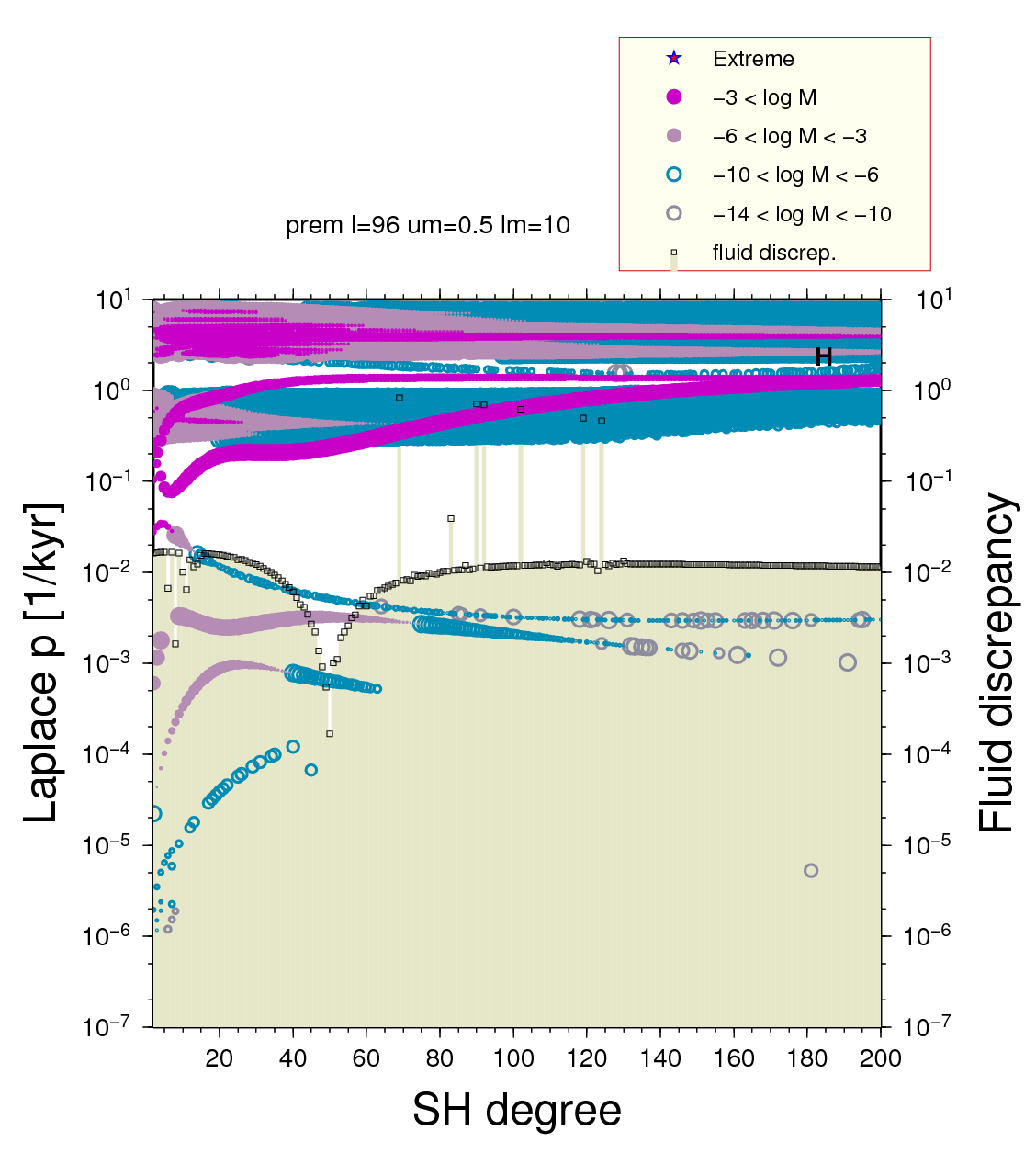
H            | -0.12512432E-05  0.13269297E-07
L            |  0.57020941E-06 -0.88461980E-08
K            | -0.10003477E-05  0.13334738E-07

Note that the first root (s = 0.43033557, log s = -0.366193) is important!
I would like to add this result to the mode file produced with the standard instruction block.
A mode-file editor is badly needed!
NEWS: We have (though a rather simple) one now, 2013-07-08.

We have another example (n=102).

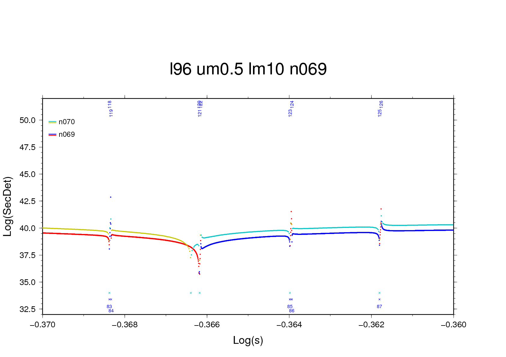
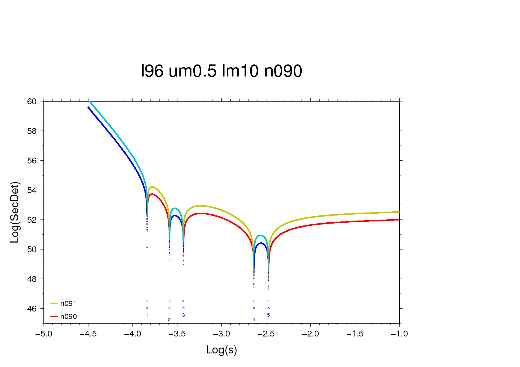
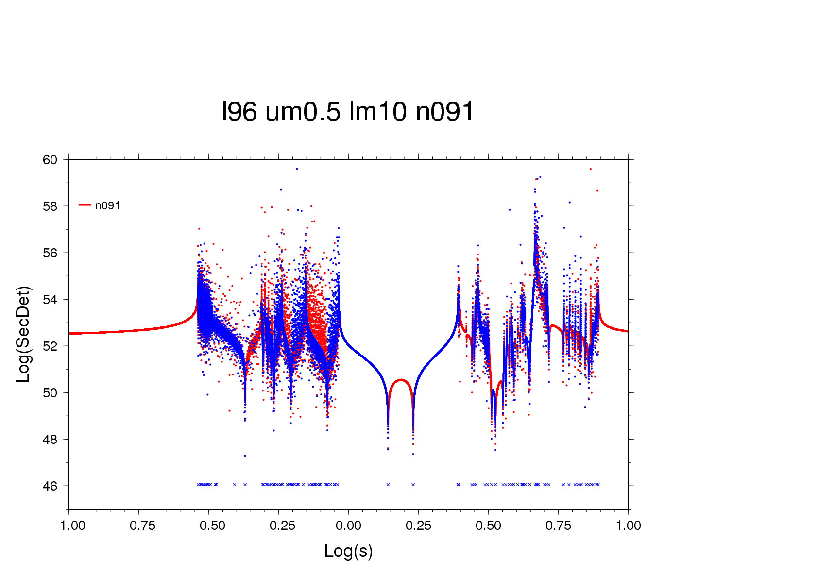
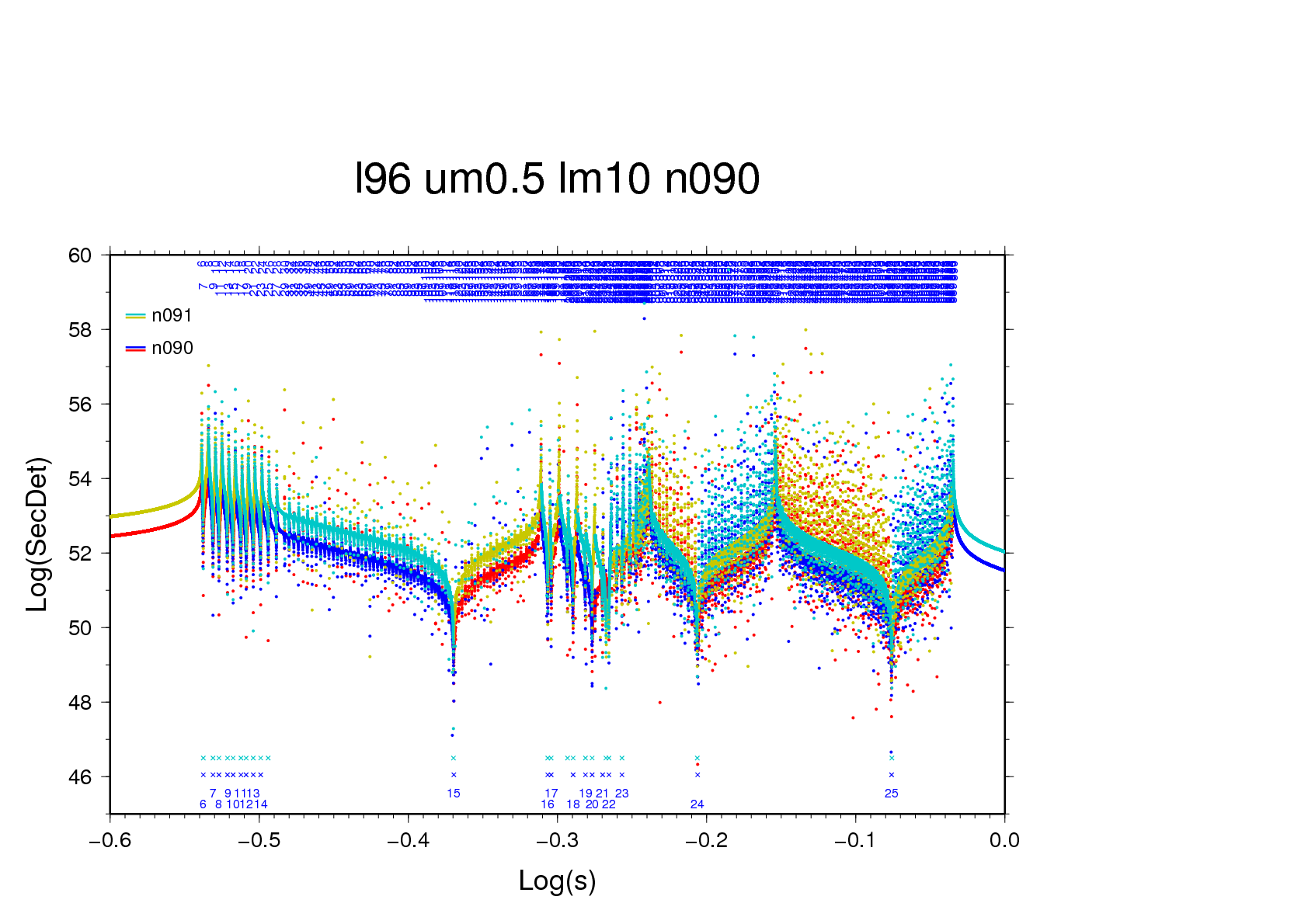
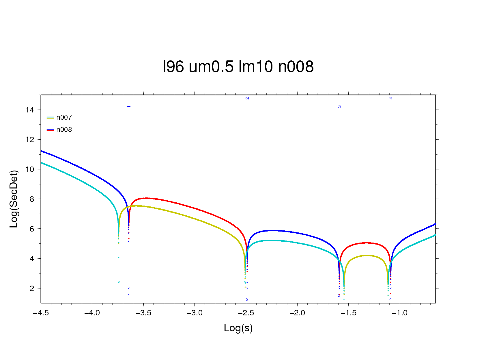
Figure 7b - using a basic scanning interval of 200,000 per decade three zero-crossings, of which one is a pole, are found near -0.3662 (n=69). With a fourfold greater interval the three crossings locate themselves within a single interval, and by mischance it's the pole that is iterated upon.


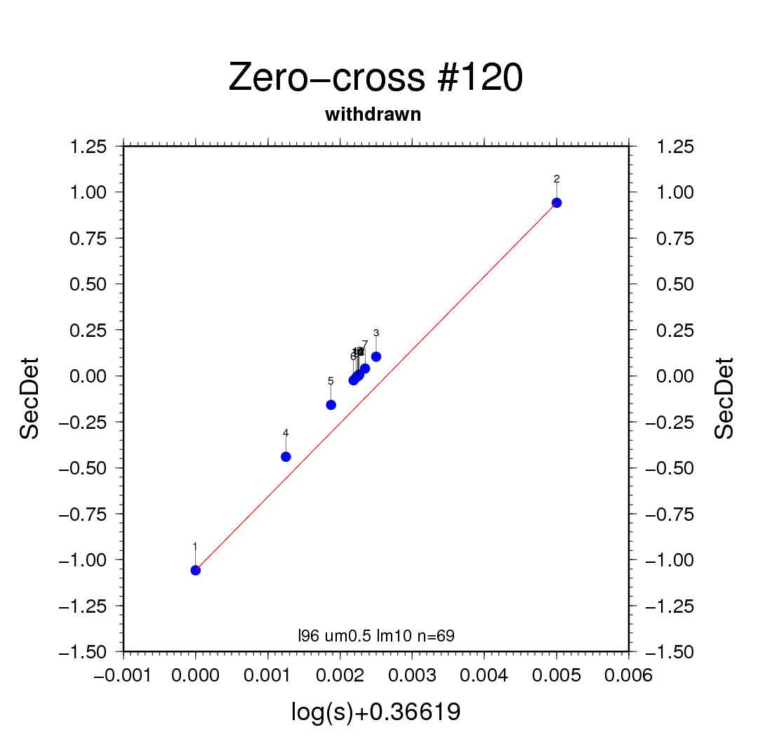
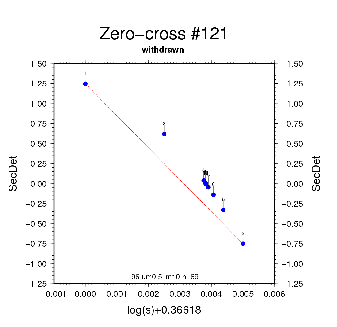
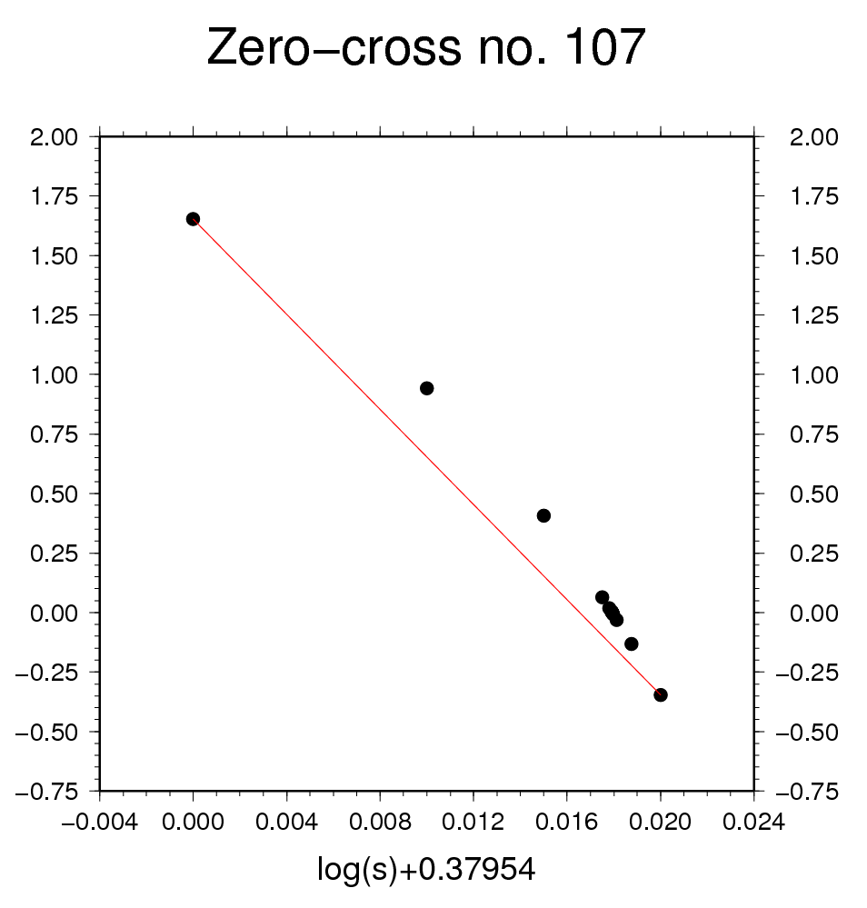
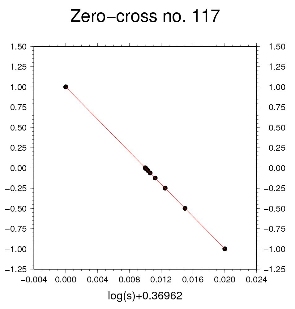
Figure 7b - even though the root is found, the series of slope values is very bumpy.


§8 - n = 2..40: Done!

Without deepening the iteration, but instead comparing slopes at bisection step 12 with the slopes at 5 to 11 (§6 @3, max [1, (Nb-7)]) the outliers in the fluid discrepancy test are gone.

This was the instruction block
: -6 -1 0.0001      1.d-12
: -1  0 0.00002     1.d-10       SLC
   0  1 0.00005     1.d-10       SLC
500 12 1.02d0  7

Final discussion and conclusions:

Inspecting the process for n=8, the root search has been looking at 605 cases and identified 300 as proper roots. One root was dismissed because of too small mode strength. 78 iterations were escaped from as the slope values decreased rapidly. The criterion for the latter (beyond the second bisection, two successive slopes differing more than a factor of 2) could be sharpened for faster processing.

At n=8 we obtain a very low fluid discrepancy. My guess is that some modes in the low-s regions are still missed. As can be seen from Figure 8b, some roots group together at narrow ranges of s, so that the basic scanning interval might still be too coarse.

In Figure 8a you can discern two mode sequences with M > 0.001 inside, respectively transgressing, the poles-and-roots band 0.1 < s < 1.0. Here, narrow basic scanning is essential.

The following three diagrams show the secular determinant for n=8 (numbered) and n=7 over the whole range  -4.5 < log s < 1. Click to see the full-scale image.


The broadband view leads me to suggest accelerating measures:
The low-s range can be scanned with a very wide basic interval.
The two high-s ranges require first a determination for their location (a few sph.harm. degrees will suffice).
The interval between the two poles-and-roots bands, where the SD is smooth, could be scanned with a wider basic interval.

Depending upon the application, the short decay times might be insignificant.

The process without these accelerations takes two minutes wall-time per sph.harm. degree on my machine.


Figure 8a -


Figure 8b -


Most recent version of the main program

.bye