Ocean tide loading explained
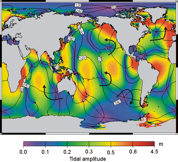
Ocean tide loading is the deformation of the Earth due to the weight of the ocean tides. The water in the ocean tides moves back and forth and these mass redistributions cause periodic loading of the ocean bottom. Since the Earth is not completely rigid, it deforms under this load and this is called ocean tide loading. One can observe it as variations at your station in vertical and horizontal displacement, in gravity, tilt and in strain. The ocean tides are produced by the gravitational pull of the Moon and Sun and since their orbits have more than one periodicities due to the eccentricity, evection and the lot, the ocean tides can be described as a sum of several ocean tides with each having their own period. The 11 periods, also called harmonics, with the largest amplitude are mostly used to compute the ocean tide loading.An example of a tidal map is given in Figure 1. The colour represent the amplitude and the contour lines indicate the phase lag of the tides with a spacing of 60 degrees.
 |
Problem areas are mostly shallow seas with large tidal amplitude and fast varying phase lag. These include among others: the North Sea, seas around Indonesia, Pantagonian Shelf, Hudson Bay and the Chinese Sea.
For more information about ocean tides see:
- Proudman Oceanographic Laboratory, United Kingdom: Introduction to tides
- NOAA/NOS: OUR RESTLESS TIDES

Here a is the loading phenomenon (displacement,
gravity, tilt
or strain) at the station located at r. The ocean
tide at r'
is given in its complex form Z=Amplitude*exp(i phase).
rho
is the mean density of sea water and G is the
Green's function for
the distance |r-r'|. The integral is taken over all
global water
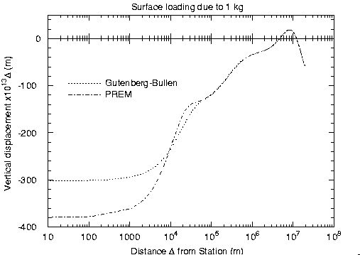
masses A. The Green's function determines how much
the Earth
deforms
due to the point load of 1kg. An example is given in Figure
2
 |
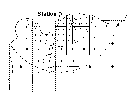
The next step is to replace the convolution integral by a summation. Most ocean models are given on a 0.5 by 0.5 degree grid which justifies direct summation over these ocean grid cells if the station is more than 10km from the coast. Otherwise some regridding is necessary. Our solution is to regrid the model gradually towards the station. Schematically this process is given in Figure 3.
 |
Of course there are other computer programs to calculate the loading. For example GOTIC2 of Koji Matsumoto, National Astronomical Observatory, Mizusawa, Japan, and SPOTL of Duncan Agnew, Scripps Institute of Oceanography, La Jolla, California.
Futher reading:
- Tides : A Scientific History by David Edgar Cartwright
- Tidal Phenomena. Lecture Notes in Earth Sciences, Springer Verlag Vol. 66, Berlin 1997. edited by Wilhelm, H., Zurn, W., Wenzel, H.-G.