Contents:
Notations:
{a,b} denotes a vector
with components a and
b
Int denotes integral, Laplace the so named second
derivative partial differential operator
{ADU,ADV} = ({CU,CV}/HV * grad) {CU,CV}
where HV is depth and {CU,CV} vertically integrated current
vector.
If terms like (CU/HV * d/dx CU/HV) would be
integrated, we would formally get terms d/dx 1/HV. This
would imply depth-dependent current variations being advected.
Most plausibly this is not the case. A formal justification for
the formulation I've decided to use is that
D/Dt Q = d/dt Q + ({u,v}*grad) Q
and Q equals Int {u,v} dz in our case, and
{u,v} = {CU,CV}/HV
Delta_CU = ... + eddy_v Laplace (CU) Delta_t
eddy_v = const.
Alternately, eddy_v = eddy_v_min * SQRT(HV_max/HV) was introduced since shallow area tides were found too high, and unreasonably large bottom friction would have been required. What could be improved (however at great computational cost) is
Delta_CU = ... + eddy_v * Int Laplace (CU/HV) dz
However, bottom topography might be too rough to expect stable results.
Advection, friction and eddy dissipation may create
difficult terms in some regions of the model. Procedures in
OTEU12.f may be used to regionally modify the model parameters.
Advection may be turned off in one region: Call
Area_No_Advection(...).
Model parameters may be redefined in one region: Call
Spec_Area(...).
The actual code of TTEQ (array PARSPA) determines the meaning of
the 10 parameters.
TEP: Tide-effective potential composed of astronomical and solid earth tide spectrum, optionally loading tides added.
ETD_SLOPE: Adding regional excitation signals to the
potential, explicitly time-dependent. In progress since
2017-08-14.
SAL: Internal self-attraction and -loading optionally by
parametrisation;
or by iteratively
adding harmonic solutions to TEP (tedious!)
APR: Sea-level air pressure fields
AB: Active Boundary tides
AB_Step: A planned step at an Active Boundary (not implemented
yet: selection of AB by name; AB-names exist already)
ntides=(index(CTIDE,' ')+1)/3
CALL Count_Packed
(FLZ,M,N,MPA)
CALL CNVCDS (ZSUM,ZSS,IWDIM,ntides+1)
NPA=1
CALL SETVER (Nsver)
FNorm=NRSUM/2.
do ih=1,ntides
j=ih*3-2
k=(ih-1)*IWDIM+1
kk=k+IWDIM
tidex=CTIDE(j:j+1)
CALL OUTZMN (41,ZSS(k),FN,MSUM,1,TYPE,TIDEX)
enddo
CALL OUTZMN
(iun,ZSS(NTIDES*IWDIM+1),FNorm,MPA,NPA,'Z','M4')
(Obsolete since the advent of solplot:) However, several procedures do not scan row number N-1 in 'Z'-arrays (e.g. ISOSCN), so either the array type should be 'M' or array dimensions MPA2=MPA+1; NPA2=2 must be used.
CTIDE - char*2 - Tides for harmonic
analysis. Specify e.g. 'M2 O1 '.
IUSAP - integer - Log.unit for retrieving tide
potential information
(OPEN done by routine).
PATH - char*32 - Path and file name for tide
potential.
NVU - integer - Number of partial
tides actually applied.
ZBUFF(NBUFF) - complex - Buffer for tide potential reading,
NBUFF = IWDIM >= number of 'S' & 'A'-cells.
H(M,N) - real - Bathymetry array.
FLZ(M,N),FLM(M,N) - integer - Flag arrays for 'Z' and 'M'
grid.
ZSUM(*) - complex - Packed CMPX array: harmonic
results for the tides specified
in
CTIDE
and,
in
addition,
the
first harmonic of the
first
tide
in
CTIDE.
More
about
ZSUM
below.
Size equal to (ntides
+1)*(number of Land + act.bound. nodes))
= (ntides +1)*IWDIM = (ntides +1)*NBUFF
where ntides = the
number of tides given in CTIDE.
NRSUM - integer - returned:
SOLVE-phase: Number of time steps used for ZSUM.
ZSUM must be divided by NRSUM/2. to yield ampli-
tudes in [m].
INIT-phases: Number of time steps to cover an integer
cycle of the basic tide (declared via Call INILTE).
ITEND - integer - SOLVE-phase: (Adjusted) time
step at end of integration.
INIT-D-phase: ... at time of dump.
INIT-0-phase: 0
In both cases:
Next time: suggested continuation at ITEnd + 1.
Call LTETIM (ITEnd+1, ITEnd+K*NCYC), where
NCYC <- NRSUM from the INIT-phase.
TGP(M,N,2) - real - Work array for tide potential, stepped in
time by
this routine.
EL(M,N,2),CU(),CV() - real - Work arrays for Finite
Difference Scheme:
Elevations, SE-, NE-currents.
EVWORK(4,IWDIM) - real - Work array for computation of
loading effects.
IWDIM >= Number of 'S'-cells.
SHOW(M,N) - real - 'M'-array, selectable grasol-show array
AUST(*) - real - Packed real
work array for Austausch coefficient.
Can be equivalenced with ZBUFF. Size >= IWDIM = NBUFF
TTEQ contains code for its own initialisation.
Before TTEQ can be called, preparatory calls are required
(code in otes01.f) in order to set model parameters
etc. TTEQ has two operating modes:
INIT (parameter preparation) and SOLVE.
INIT has two submodes:
INIT from scratch (INIT-0);
INIT from a dump (INIT-D).
During INIT-0 - and only there - the
time step length is determined.
INIT-D and INIT-0 return the tide cycle length and the
previous closing time step number (ITEnd) through the TTEQ call
list (variables NRSUM and IT).
SOLVE should continue at ITBeg := IT+1 and close
at ITEnd = IT+KCYC*NRSUM after INIT-D.
SOLVE should start at ITBeg = 0 and close at
KCYC*NRSUM after INIT-0.
Code is in otes12.f
(alt 1) specify a measure for the
subcriticality, a factor on the critical time step. A
subcritical step is shorter. The closer the time step to
criticality the more exact is the solution (theoretically; this
statement is only valid in the deepest part of the model);
CALL INILTE
(0, Subcriticality_Factor, Basic_Tide_Symbol) ! for
instance...
CALL INILTE
(0, 0.99, 'S2')
(alt 2) specify the number of time steps in one cycle
of the basic tide:
CALL INILTE
(N_steps, 0.0, Basic_Tide_Symbol)
(alt 3) a rounded alt. a fixed step length. In case
studies where complete harmonic cycles aren't an issue, the time
step can be rounded to integer seconds; or a fixed value can be
specified:
CALL TTEQ_ROUND_DT
(QRound_Dt, Fixed_Dt)
Qround_Dt .true. will take precedence, else Fixed_Dt
is accepted if > 0.
TTEQ differs from LTEQ on the part of the designation
of ITBegin and ITEnd. It is advantageous to use the
S2 tide as the basic tide, which determines the step length of
the finite difference scheme. The program can be made
synchronous with a UT-clock, thus generating output series for
tide gauges and CrustalDynamic Sites at exact hours.
Recipe: Run a first test (which you will
abort) with
DOUBLE PRECISION DT1, DT_LTE
...
CALL INILTE (0, 0.999, 'S2')
CALL TTEQ (...
DT1=DT_LTE ()
to obtain a near-critical time step, DT1. Abort the
program, and choose next time
CALL INILTE
(n, 0.0, 'S2')
where
n >~
IDINT(((12*3600)/DT1 + 1)/12)*12,
This gives a near critical time step which divides one hour integer.
However, the tide subjected to harmonic
analysis does not have to be the S2 tide. In that case, ITEnd =
IT+KCYC*NRSUM does not provide an integration interval
that covers complete tidal cycles, and the harmonic analysis
result would become perturbed. Therefore, use
CALL TTEQ_ADJT (.TRUE.)
to obtain a complete last cycle of the tide first stated
in the CTIDE string, so that its harmonic solution is
as accurate as possible.
The loading part requires a separate initiation (INIEVL_ETD).
The other packages engaged by TTEQ (like the tide generating
potential) allow/require parameter setting from the calling (the
main) program.
| Index |
RGP |
QGP
if (.true.) then ... |
IGP (no,
this is KSGN in otes18.f) |
|
| 1 |
Cut the phase
circle at this angle (degrees), used in graphics display and printed results of harmonic solutions |
Array selector for graphic trace 1) |
||
| 2 |
Scaling factor
for advection term; 1.0 means the
full effect. |
Harmonic
solutions are requested for Z-array |
Stop at this time step 2) | |
| 3 |
Effective
Coriolis is RGP(3)*FCORIO*DTN, 1.0 means the full effect. |
Harmonic
solutions are requested for M-arrays (mutually exlusive with QGP(2)) |
Upper harmonic selector to show 2) | |
| 4 |
Harmonic
analysis is to include DC-level |
|||
| 5 |
Also analyse
the first upper harmonic |
|||
| 6 |
||||
| 7 |
||||
| 8 |
||||
| 9 |
||||
| 10 |
Detect NaN's |
tide
forcing
(OTES17*.f)
tide gauge and crustal
loading
(OTEU16*.f)
air pressure
forcing
(OTES15*.f)
special areas (modified model
parameters) (OTEU12.f)
user
interaction
(OTEU18.f)
graphic
display
(OTES18.f)
buoys
(OTES19.f)
Several of these allow/require parameter-setting calls.
Execution
options:
Reset
ZSUM,
Graphics,
Write
state arrays
To be called before the iteration is started:
CALL LTEOPT (OPTION)
LTEOPT -
options:
OPTION - char*3 =
'rgw' where
r
- 'Y' - reset ZSUM before LTEQ-time stepping,
'N' - don't ... '.' - unchanged. Default = 'N'.
g
-
'A'
'E'
'a'
or
'e' - graphic display of tide elevation on-line.
Capital letters for prompting
mode enable.
'A' 'P' 'a' or 'p' - graphic display of tide generating
potential.
Capital letters for prompting mode enable.
'N' - don't ... '.' - unchanged. Default = 'N'.
w
-
'Y'
-
save
state
arrays
on
file,
log.unit
2,
for later
resuming of iteration.
- 'O' - rewind the file before save.
- 'N' - don't save.
- '.' - unchanged. Default = 'N'.
Some parameters are stored in the dump; their values can
only be changed after the INIT-D calls and before the SOLVE call
to TTEQ.
(Mark = >D< )
Parameters which must be given before the SOLVE-call :
(Mark = >S<)
The friction parameters are not stored; thus CALL LTEFRI
must appear before SOLVE calls. Subsets of parameters can be set
by alternative calls.
CALL SETLTE (T_beg, T_end, FRIC, NF_cons, TF_relax,
NF_end, NRAMP,
I_mon, J_mon, OPTION)
LTETIM -
parameters:
>S<
T_beg, T_end - integer - Model start and end time;
preferably
T_end - T_beg. + 1 = K * (tide.period)/dt. C.f. above
"Start from an initial solution" how to obtain the
the integer value: (tide.period)/dt
CALL LTETIM (T_beg, T_end)
LTEFRI - parameters: Friction / damping and control: >S<
Run-in phase = damping. Uses parameters
FRIC(1), NF.cons, TF.relax, NF.end.
Physical friction model: FRIC(2..4);
dt = used time step [s], check protocol.
FRIC(1) - Friction coeff.
for damping during start-up
dM/dt = p M abs(M)/Hmax. FRIC(1)= p dt = O(0.1)
FRIC(2) - Linear bottom
friction parameter.
dM/dt
=
-
r
M,
[r]
=
1/s.
Here
FRIC(2)
=
r dt, hence
FRIC(2) should be O(0.1)
FRIC(3) - Quadratic bottom
friction parameter.
dM/dt
=
-
q
M
abs(M)/H.
FRIC(3)=
q
dt,
e.g.
=
0.3
FRIC(4) - Eddy viscosity
parameter. Check the code in OTES12.f
how eddy visc. is formulated (depth-dependent ?).
Reasonable values are between 1.e4 and 5.e5 m**2/s
dM/dt = + v Laplace M, FRIC(4) = v (!)
FRIC(1..4) - real, dimension=4. Values must
be >= 0 to be accepted.
Zero value switch the mechanism off.
NF_cons - integer - Time
step until which run-in damping is
kept constant.
TF_relax - real - Relaxation
time (model units of time) for
exponential decrease of FRIC(1).
NF_end - integer -
Time step after which FRIC(1) is 0.
CALL LTEFRI (FRIC, NF_cons,
TF_relax, NF_end)
LTERMP - parameter:
>S<
NRAMP -
integer - Duration of raised-cosine ramp. The driving
forces are turned on during the start-up phase using
a raised-cosine ramp. NRAMP is specified in model
dt-units. No default.
CALL LTERMP (NRAMP)
LTEMON - parameters:
>D<
I_mon, J_mon - integer - The position X and Y of a mesh
point at
which characteristic values will be printed during
time stepping. No defaults.
CALL LTEMON (I_mon, J_mon)
PARLTE - parameters
(p1,p2,p3,p4,q1):
>D<
p1
- real - Hmin, the minimum depth for bathymetry. The
array H(i,j) will be adjusted. Default = 5.0 (meter).
p2
-
real
-
WDT_fric,
the
time
offset
inside
dt
at
which
the
friction terms are defined; counted from t+1 backward.
WDT_fric=0.0 <=> t+1,
WDT_fric=1.0 <=> t. Default = 1.0
which is also the "classical" definition.
p3
- real - G_fac, a factor multiplying gravity. It was
found
that
an
increase
of
g
->
1.1
*
g
improves
the
fit of the discrete dispersion relation w.r.t. the
continuous case. It's doubtful though. Default = 1.0
p4
- real - SLP = self loading parameter. Applied as
EL_eff = EL * (1-SLP). Default = 0.0
If a default value for p* is to be used, specify p* <=
-1.0
q1
- integer - NONLIN-earities.
< -1 - default: shallow water
-1 - don't change
0 - linear
1 - shallow water (=default)
2 - advection
3 - 1 & 2
CALL PARLTE (Hmin, WDT_fric,
G_fac, SLP, NONLIN)
INILTE - parameters:
N_steps - integer - Number
of time steps per tidal cycle.
Default = 0, i.e. P.subcrit is used to determine the
time interval.
P_subcrit - dt = P * dt.crit is used;
dt will be further adjusted
downward such that the tidal cycle is divided into an
integer number of steps.
Default = 0.75
TIDE - char*2
- The tide that determines the fine-adjustment of
the time step.
CALL INILTE (N_steps, P_subcrit,
TIDE)
N.B.: INILTE resets the PARLTE - parameters.
General Parameters (special
extensions):
CALL SETLTE_QGP (i,qq)
CALL SETLTE_RGP
(i,rr)
CALL SETLTE_IGP
(i,kk)
where i has type integer, qq logical, rr real, and kk integer.
Some SETLTE_*GP settings are ready to use:
______________________________________________________________
i Meaning of _QGP qq
--------------------------------------------------------------
1 Use a depth-dependent
austausch coefficient
(qddaus in
otes12.f) Feature is presently
disabled
(commented out with 'ccc' ).
2 Accumulate harmonic from elevation field
3 Accumulate harmonic from current fields
4 Accumulate DC-level
instead of upper harmonic
______________________________________________________________
i Meaning of _RGP rr
--------------------------------------------------------------
1 phase cut (usually 0.,
could be 180.) for the harmonic
trace graphics showing the
phase field
2 factor on the
advection terms (should be 1.0)
______________________________________________________________
i Meaning of _IGP kk
--------------------------------------------------------------
none implemented as of 2011-03-11
Also, 2 and 3 are mutually
exclusive, and if the program finds
both true or both false it will set 2
true and 3 false
RTRLTE - parameters:
N_save - integer -
Resume with the N'th saved solution from file
on
log.unit
3.
If
the
file
contains
L
sets,
L
<
N,
the L'th will be taken.
N_cont - integer -
Number of time steps to continue. C.f. above
"RESUMING A PREVIOUS SOLUTION" for advice how to obtain
LTETIM parameters if an appropriate value is not known.
CALL RTRLTE (N_save, N_cont)
TTETEP -
parameter:
>?<
N_steps - integer - Update
interval (number of time steps) for the
tide effective potential. Linear interpolation between.
Default = 20
CALL TTETEP (N_steps)
LTETDS -
parameters:
>?<
N_steps - integer -
Interval between on-line display of elevation.
Default = 42
range -
real - The data range [m].
Default = 1.0
Inquiry:
= DT_LTE() - Real*8 entry DT_LTE()
returns the time step length [s]
CALL
EXTCTP
to extend common block space tide potential
CALL
EXTCTO
to extend common block space global load pot.
CALL
EXTCTA
to extend common block space active boundaries.
CALL
ETDSEL
to select partial tides for forcing
CALL ETD_NO_BODY_TIDE
CALL ETD_NO_LOAD_TIDE
CALL
ETD_ABZ_TIDE
(de-)select active boundary forcing
CALL
ETD_ABZ_Factor
to amplify active boundary tide
Tide forcing, parameter
setting (OTES161.f)
-------------------------------
CALL
ENABLE_PLAY_WITH_ETD to enable
code in subr. PLAY_WITH_ETD
Simulated air pressure forcing: (OTES15*.F)
-------------------------------
CALL
Pressure_Param
to define size and velocity of a model pressure system
CALL
Pressure_Stop
to stop simulation
CALL
EXTABP
to extend the buffer for act.boundary data.
To force
with actual met fields, use otemw1.f
Regional excitation:
(OTES17.F)
--------------------
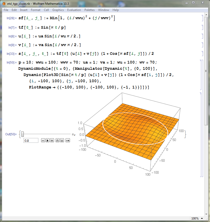
CALL ETD_TGP_SLOPE (string) 'E:<four
parameters>'
for east-west geometry
'N:<four
parameters>'
for north-south "
'T:<three
parameters> [options]' for
timing, event ahead
'T!<two
parameters> [options]' for timing, launch event
now!
'.?'
inquire status
'RESET'
switch off
See details on parameters here.
The update interval for the TGP should be set at a small value;
without tides and loading, the computational burden is
negligible.
The namelist parameter in otemt1.f is IDTTEP , setting
the number
of diff-eq. time steps to lapse between calls to ETDCMP.
More on active boundaries: (OTES13.f)
--------------------------
CALL
FREEAB
to free the inner row of elevation boundary
CALL
ETD_ABZ_Step
to force model with unit step
CALL
ETD_ABZ_EAPR
to maintain inverse barometer at act.boundary.
Tide gauges (OTEU16.f)
-----------
CALL IUN_TIDE_GAUGE
CALL ADD_TIDE_GAUGE
CALL SAFE_TGG
CALL
IUN_TGP_SENSOR
to output time series of tide generating potential
CALL ADD_TGP_SENSOR
Crustal Dynamics Sites (Loading effects) (OTEU16.f)
----------------------------------------
Calls in that order:
CALL
ADD_EVL_SITE
add sites
CALL
IUN_EVLOAD
define output file unit
CALL
ISOFOR
define what boxes to be included in load scan
CALL
INIEVL_ETD
initialize load routines.
Buoys (OTES19.f)
-----
CALL
SET_BUOY
add buoys
CALL
IUN_BUOY
define output file
CALL SAFE_BUOY
CALL
DO_BUOY
activate time-stepping
Special_Areas (OTEU12.f; user interaction: OTEU18.f)
-------------
CALL AREA_NO_ADVECTION to avoid advection term in a limited area
CALL
SPEC_AREA
to define an area with alternate parameters
CALL
SPEC_AREA_PARAM
to set parameters
Use of Spec_Area parameters is flexible. Currently:
Parameter(1) factors
the bottom friction terms, P(2) the eddy term, P(3) is a
minimum depth.
Graphic display
---------------
CALL
GRASOL_DS
to display double size color pixels
CALL
GRASOL_SS
to display single size
The operator may interact with TTEQ. Notice: may. A good,
stable solution will rather be one that thrived without the
intervening hand of a person. However, some features have been
included which allow changing of parameters as the program steps
along.
There are two routes of intervention, from a console window
(this chapter), and the Graphic Display Prompter
at the graphic screen.
The graphic screens, especially the Trace
feature, allows mainly logistic interaction. For example, an
Active-Boundary step experiment can be initiated from the
graphics window.
When
numeric values are expected and you prefer a default value,
hit the Escape-key. The Return key will keep you in a loop. (The functions used are int_prompt_s18
and real_prompt_s18
.)
On the PC the program scans the keyboard directly. On the
UNIX platform, however, the program reads a little communication
file. The user writes characters into this file using the OC command.
Use OC
from another terminal window or run TTEQ-SOLVE in the
background; redirect output for convenience.
Example OC ^M : do spell out the two
characters, "Caret M" instead of the composed key press CTRL+M
on the PC.
Since xterm under Cygwin on a reduced keyboard (laptop)
frequently loses the delayed-compose key '^',
a backslash can be used instead. Unfortunately, the OC parameter must be put
inside quotation marks, e.g. OC '\E'
Code
^@
The date and time of
the next step are written to the protocol.
^H
The table header is
printed on the protocol
^M
The program waits for entries that modify the Spec_Area. C.f.
oteu12.f and oteu18.f
^D
The depth array H(m,n)
can be updated.
^E Prompt
after the next display of the elevation array
^F The friction parameters FRIC(1..4) can be adjusted.
^V
The system asks for new
monitor node position (enter at text prompter
on
graphic screen).
^W
^X "when?" - the ending step will be
printed on the protocol and the
grasol
status line.
^X:
Grasol will prompt (cannot display the status then). Taken out of service
^W Write the three
arrays to file (E -> iun_save , Mu & Mv -> iun_save+1)
iun_save
is set with call tteq_save2unit(i) .
Default=91
The
arrays can be plotted using elplot
and uvplot
^S
The program stops after
writing the dump file.
^Z
Some general purpose
parameters. E.g. parameter 1 means the
phase cut
parameter. Phase is shown in graphic trace of harmonic
solutions. The input of a new value is carried out at the
graphic
prompter. See otes12.f at "^Z - special purpose"
^Q
The program stops immediately.
Other user interactions concern screen graphics and tracing.
^A Trace of active boundary data is initiated for the next time step.
^O Trace of etd-o-o-area data is initiated for the next time step.
Graphic displays can be modified in a number of ways. Irregardless how OPT(2:2) was declared at call time...
^G
The elevation array
will be displayed and prompt after display
will be
reactivated.
^P
The tide generating potential
will be shown and prompt after
display
will be reactivated.
^T
The graphic trace is
switched on and prompting after display
will be
reactivated. Time step for next graphics is set to 1.
^U
Like ^T, time step is unchanged, however.
A nice feature is that you can watch the harmonic solution as
they (hopefully) converge. Do the following:
From the outside, OC ^T
At the graphic prompter, choose c and 18
to select phase, I and e.g. 100 for
the time increment to redraw, finally G
for go,
then watch.
If you want to show another constituent (provided it is enabled
through calling parameter CTIDE), do
^T
, enter # at the graphic prompter (not in the menu) and
type 1 for the second tide in
progress.
More details in the next chapter.
New features have been included in the OC
mechanism:
Control of model excitation
of the ETD_TGP_SLOPE kind.
Function UBR_FF (oteu18.f) will
interpret the '!<command-string>' argument
and call ETD_TGP_SLOPE(string).
OC '!S <command-string>'
e.g. for an est-west slope centred on grid
index 145, height 1.0, half-wave length 350 units, tapered at
twice the length,
acting with a period of 30 hours, for the next
30 hours ahead (half-period but sine-squared!)
OC '!S E:1.,145.,350.,2.'
OC '!S T!30.,30.'
An aid for parameter specification is here: http://holt.oso.chalmers.se/hgs/OTEQ/etd_tgp_slope.nb
(Mathematica notebook; see png-image
(prefer to open it in a new tab/window)
OC '!E <file-unit,modulus>'(both must be given; a file must have been opened in the file-open block)
OC '!F <n>' - sets subtype nIn GraSol, the corresponding command keys are F, T and V and their lower-case versions.
OC '!f' - recalls subtype scanning.
OC '!T <flags>' - sets a new target string. If non-nil, sets it permanently (calls ISOFOR).
OC '!t <flags>' - sets a new target string for the next instance of GraSol.
In order to abort integration if the system turns out unstable,
this feature surveys the solutions and warns (protocol), reduces
the repeat interval of graphics to one step. When a severity
threshold is exceeded, it will stop the process. Code is in
oteu12.f . Watchdog options, CALL...
WATCHDOG_CLIP(xl) - essentially an illegal and worthless action: clips the array at these limits (-xl .. +xl)
WATCHDOG_MOD(n) - how often the array is observed (n = modulus of time step number; if zero, analyse)
WATCHDOG_BITE(xx) - stop when absolute value of any node value exceeds xx.
WATCHDOG_BARK(x) - warn when absolute value of any node value exceeds x.
WATCHDOG_POINT(q1,q2) - if q1 is .true., set immediate reactivation of graphics according to q2. Effectuated with "bark".
Table
GRAPHIC TRACE -
Component numbers and the variable that is traced
To select the array, press the f
or c key
at the graphic prompter and enter a number:
| 0 | Friction/damping scaling factor |
| 1 2 | Coriolis terms in U and V, respectively |
| 3 4 | Gradients of tide generating potentials along x and y directions, respectively |
| 5 6 | Advection terms along x and y directions, respectively |
| 7 8 | Eddy viscosity terms along x and y directions, respectively |
| 9 10 | Mass transport vector M = {U,V} |
| 11 12 | Current vector M/h |
| 13 14 | Friction force along x and y directions, respectively |
| 15 16 | dM/dt |
| 17 18 |
Harmonic solution,
amplitude (17) or phase (18). Select a specific
constituent with the #
key |
| 21 |
(not finalised yet) Show the tide
generating potential (not the gradients). Problem is that
the flag array used is type M, the TGP array is type Z. |
| Return
to Displays | Return
to Displays grasol prompter |
The display and prompting occurs in subroutine GRASOL (/home/hgs/Oload/p/gra/otes18.f)
<CR> Pressing the Carriage-Return key satisfies the GDP. TTEQ will continue.
I Press "I" (Increment option) and define the number of time steps until the next display.
G
T
"Go" and "Text screen" modes are toggled modes (key "G"
or "T").
Go means that
the prompter is skipped. (Regain control by e.g.
sending OC ^G
from the outside.)
Text
screen
should
be
selected
if
graphic
mode
is
undesirable between consecutive maps.
S
Stop mode (S-option) implies skipping the display
routine; you can re-enable
the display mode by sending OC ^E, OC ^P, OC ^T or OC ^G, depending on
what you want to see.
Pressing "S" passes control to TTEQ.
d Dump the elevation array
to real-binary file. The system prompts for a file name.
Enter a file name containing
one `#´ character, and the dump will recur with
every array shown.
The `#´
character will be replaced by the step number.
(careful! Request only one
array variable for show!)
Enter a `.´
character to stop dumping.
r
The data range can be changed: Press "r" and enter a
new value. The data range
may
optionally
be
clipped
against
the
color
range;
this
option
is always prompted for
before you are asked to enter the range value(s). Press "R"
and redefine the
data
range
to
be
one-sided,
two-sided
or
general
(-1,
0,
+1). In the second case you need
to
enter
two
values,
for
the
lower
and the upper range, respectively.
Overrange colors are difficult to interpret. Lower-than-bottom is
shown by
mixing
black
and
a
base
color,
higher-than-top
by
mixing
base
colors that
are
two,
three,
...
intervals
apart.
The
color
numbers
are
derived with
the MOD function; thus, vastly-out-of-range data will still be
colored
quite similar to inside-the-range data, and is hard to discern.
After changing the data range, the map is
redrawn.
l h Press
l
to get low resolution, h to get
double size pixels.
1
2
Synonymes: 1
and 2. Larger numbers will draw larger cells;
maximum size is 7.
L H
Press L or H
to cause the screen to be refreshed while changing resolution.
a A Press a to redraw, A to refresh the screen.
V
Press V
to redefine the target symbols for display. This redefinition
is valid only during the subroutine instance.
^C Pressing ^C at the GDP stops TTEQ; the routine requests confirmation before it will dive.
c f Press
"c" to get prompted for one of 10 integer
parameters to set.
Press "f" to set the first
parameter right-away.
#1
-
Select
a
component
to
show;
cf
Table GRAPHIC TRACE.
#2
-
Set
the
terminating time step of the the on-going TTEQ cycle. The actual
time step is shown in the purple status bar.
#3 ... unused.
Selecting 17 or 18, a tide harmonic solution in the making, will
re-activate the graphic screen at every zero-crossing
of the imaginary part of the Fourier factor.
#
Press "#" after selection of
component 17 or 18 to request view of a specific harmonic
solution. You can
watch
the
convergence
of
the
solution.
In
the purple status bar you can check the exp(wt); if it is (1,0),
a
harmonic
cycle
for
the
wave
in
question is complete and the solution relatively well-determined.
Enter 1 for
CTIDE(1:2), 2 for CTIDE(4:5), ntides+1
for the double-frequency nonlinear tide.
If
you
e.g.
asked
for
two
harmonic
solutions, enter 2 and you'll see the
double-frequency solution of
CTIDE(1:2) (e.g. M4 if CTIDE = 'M2 O1 ') .
@
Press "@" to get
prompted for a halting time. At the halting time the graphic
display will be
revived and stay in prompt mode (ithalt_grasol()
function)
/
Plan an Active Boundary Step
experiment. Respond to the following prompts:
Start
and
end
of step: How many time steps ahead (end: default=indefinite)
Step
height
(default:
1.0) Press ESC for defaulting.
^S
Press "CTRL-S" to set
up a SPLASH test. System
prompts for location, strength, time and duration
Start from a zero state:
using SETLTE common using LTE***(1) Read arrays H, FLZ, FLM
(3) CALL SETLTE (0,-1, CALL LTETIM (0,-1)(4) CALL PARLTE (p1,p2,p3,p4,q1) optional
FRIC,NF_cons,TF_relax,NF_end, CALL LTEFRI (Fric,NF_cons,TF_relax,NF_end)
NRAMP, CALL LTERMP (NRAMP)
Imon,Jmon, CALL LTEMON (Imon,Jmon)
OPTION) CALL LTEOPT (OPTION)
(8)
ITBegin = 0
ITEnd =
K*NRSUM
! e.g. K = 6
CALL LTETIM (ITBegin, ITEnd) ! SOLVE call
CALL TTEQ (...)
______________________________________________________________________
Resuming a previous solution at t = T :
(1) Read arrays ZOTEP, H, FLZ, FLM
(2) CALL RTRLTE (N.save, NT.cont) ! INIT-D calls
CALL LTETIM
(0,-1)
!
CALL TTEQ
(...,IT,NRSUM,...) !
(3) ITBegin = IT+1
ITEnd =
IT+K*NRSUM
! e.g. K = 6
(4) CALL LTEFRI (...)
and, optionally, other LTE*** routines,
incl. PARLTE
(5) CALL LTETIM (ITBegin, ITEnd) ! SOLVE
call
CALL TTEQ (...)
______________________________________________________________________
.bye