The spatial domain is a flat earth approximation with some
(hopefully
the
most important) earth spherical effects or consequences of
geometry
being
mapped. The different fields are gridded (discreteized) in a
special
fashion
following the work of Sielecki (1968) and Wübber and Krauss
(1979).
Mapping is by stereographic
projection. Procedures are available at
/home/hgs/OTEQ/s/oteu011.f
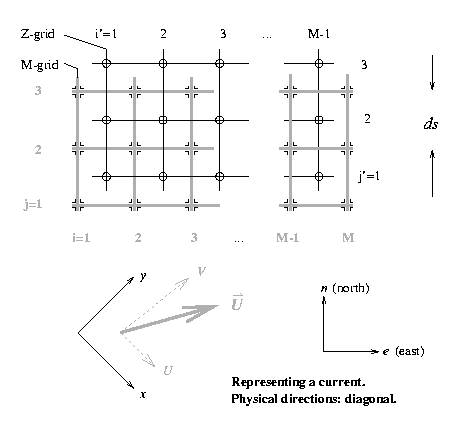
The fundamental directions in a physical sense (x,y) are
along
the diagonals of the grids.
The grid representing the currents is given the type code M, the
one
for elevation the type
code Z. The Z-grid has one row and one column less than the
M-grid.
However, for
file reading/writing we will input/output MxN
elements, though there will be M+N zeros
when we process a Z-grid.
Ocean depth, currents (and eventually surface wind) are
represented
on the M-grid;
elevation, tidal gravity potential (and eventually air pressure)
on
the Z-grid.
In the scientific texts we can distinguish the two grids by
unprimed
and primed index
numbers, i.e. i,j on the M-grid and i',j'
on the Z-grid.
The position of a grid point from the origo (centre of the area)
in
kilometers e - east
and n - north is given by
e = [i-(M+1)/2]*ds, n = [j-(N+1)/2]*ds (M-grid)
e = [i'-M/2]*ds, n = [j'-N/2]*ds (Z-grid)
where ds is the grid constant. In the
programs
it
is usually termed SCALE and its
numerical value is given in kilometers.
Flag values may show three things:
(1) represent a circumstance (e.g. land/sea)
(2) indicate a specific kind of boundary condition
(e.g. a straight piece of shoreline
running north-south
with sea to the east)
(3) specify a storage address for memory-efficient storage of
auxiliary data (mostly the tide
height
along an open boundary)
Some basic facts:
Passive boundary conditions are associated with land.
Passive boundary conditions apply only to the equation of the
currents.
Out-of-area nodes need only a distinction between land and sea.
An active (open) boundary is associated with sea.
Passive boundary conditions may occur on the end members of a
segment of active boundary, where it eventually
touches
land.
Using open boundaries a model can be driven by elevations or
currents or a combination (compatibility needs to be
established
though).
The boundary current case, however, is rare since
such
data is usually rare
or uncertain or noisy.
See more under Passive boundaries or Other flags.
Tide excitation: Recommended program has name otemt1, document names otemt1.doc and otet.doc. Code is available at geo/hgs/PC/OTEQ/EXEC/otemt1.f
Pressure and wind excitation: Recommended program has name otemw1. Code is available at geo/hgs/PC/OTEQ/EXEC/otemw1.f
Static pressure loading: Recommended
program
has
name apload.
Code
is available at geo/hgs/PC/OTEQ/EXEC/apload.f
See the pages about general aspects of files
and displays.
.bye