- Selecting
files by weekday
- RAW data |
- 1-min
gravity, baro, predicted tides -> MC |
- 1-s gravity ->
BIN ts
- 30-s MC ASCII from G1 |
- 10-min data
from G1 | 10-min
data from e.g. garb MC |
- Empirical residual
- Polar motion
data: |wget IERS
data; extend eopc04_IAU2000.orig; compute gravity
- Subtract polar
motion: | see item 7.
- Drift
determination: | tide analysis, air
pressure, polar motion reduction
- Tide analysis |
- Gravimeter:
sliding residual RMS |
- Tilt controllers: | sliding RMS and long-term drift; and a
power spectrum.
- Si Diode
thermometers | at the
coldhead ("neck")
- Plot | Plot many curves |
- GGS | 1-s data for mode detection
and ftp to GGP
- Free Oscillations |
- Daily
residuals, micro-seismic spectrum, shocks, and cleaned
low-rate data |
- Daily
RMS |
- Daily PSP |
- A
sequence of periodograms |
(every hour for 1 day, 1-s data) is an example in the tslist man page
- Determine the daily "human"
signature (working days versus holidays)
- A diagnostic plot with
GMT |
PRELIMINARIES:
File types
.tse - time-series edit
control, c.f. tsfedit,
a fortran subroutine called in e.g. urtap
(tide analysis) and tslist (time series utility)
.ins - instruction files
for most fortran main programs
.ts - binary
time-series
.mc - binary multi-component
time-series
.dat and .tsf: ascii
Useful utilities:
Those in bold with no
http-link should display help text upon option -h
GENERAL:
urtap
urtip tslist (tsl) tsd JDC
jdc(-v2)
YMD sasm03
sasm04 sasm06 sasm08
also see File utilities
and TS-utilities.
Cron jobs:
get-tide-data
yesterdays-G1-plot
tide-press-plot actual-memsp-vs-time
GGP-send-data
pt4brimer
monthly-600s
tilt-control-monitor
longt-gbres
GRAVITY / MEASUREMENT:
ggpheader.pl prep-ggs
xchan-units
SPECIAL: ~/TD/
irreg-in-raw
app2days tslapp
bzip_or_rm daily-psp
daily-resid daily-rms detect-shocks
fo-spectrum lpf-ts2ts myfo
useisp
MAKEPMG polmotm
resids
run-daily-psp-vs-time
run_urtip SCG2ts tiltrot
ts2mc-resid
tsf2ts-decim
useisp
vartst.pl
xggp
PLOT:
plot-psp-vs-time
tsld tslg
PLOT:~/TD/plot/
hans-tsplot.env
plot-psp1f-vs-time
psp-plot
hms-plot
t
tcsh source scripts:
~/TD/plot/
3sp.env hans-kattegat-tsplot.env
hans-rms-tsplot.env hans-tsplot.env
rastered-pdg.env wx-mcplot.env clear.env
hans-mcplot.env
hans-spplot.env
mcplot.env tilt-xy.env
documentation for these is badly needed!
A1 AND A2 FILE TYPES, CHANNEL
SETUP:
xchan-units -c RAW_o054/A2100102.054
Channels
1
2
3
4
5
6
7
8
9 10
0
LHe-Lvl AGnd
AD-1 AD-2 G1-Sig
G1-Mode G2-Sig G2-Mode
Dewr-P GBal-1
10
TX-Pwr TX-Bal NeckT-1 NeckT-2
BelyT-3 BodyT-4 LHeLvl
GBal-2 TY-Pwr TY-Bal
20 Tmp-Bal
HtrCrnt Temp-6K Temp-77 FB-Mod
P1GasCl P2GasRg P3CmpHi P4CmpLo P5CmpBl
30
T1-Ext T2-Ext T3-Ext Temp-G1
Temp-G2 Temp-TX Temp-TY Temp-TE
Temp-AX Temp-CH
40 Temp-Gt
Dwr-Htr Comp-DC CH-DC
Tmpr1 Tmpr2 RelHum1
RelHum2
xchan-units -c RAW_o054/A2120222.054
MRS: 9999.999
Channels
1
2
3
4
5
6
7
8
9 10
0 LHe-Lvl
AGnd AD-1 TREEfan
G1-Sig G1-Mode G2-Sig
G2-Mode Dewr-P GBal-1
10 TX-Pwr TX-Bal
NeckT-1 NeckT-2 BelyT-3 BodyT-4
GBal-2 TY-Pwr TY-Bal Tmp-Bal
20 HtrCrnt Temp-6K Temp-77
FB-Mod P1GasCl P2GasRg P3CmpHi
P4CmpLo P5CmpBl T1-Ext
30 T2-Ext T3-Ext
Temp-G1 Temp-G2 Temp-TX Temp-TY
Temp-TE Temp-AX Temp-CH Temp-Gt
40 Dwr-Htr Comp-DC
CH-DC Tmpr1 Tmpr2
RelHum1
RelHum2
Merging two RAW files for the same day
~/TD/
merge-RAW -h
Test for
differences daily-mean values for all channels in an A1 file
Two days, here July 1, 2009 and Dec. 1, 2010, retrieve all 48 channels
tsf2ts-decim -w -r 1 -u 1-48 -o d -d 1 RAW_o054/ A1
0907
tsf2ts-decim -w -r 1 -u 1-48 -o d -d 1 RAW_o054/ A1
1012
Print a table of differences of daily means
chancheck 'd/A1_*_101201-1m.ts' 'd/A1_*_090701-1m.ts'
A hi-quality 1s to 1 m decimation filter:
FILTER D:WD
KAIS 480 2.5 30 0.0 0.34 0.
Window design
half-length 480 (16 min full duration)
KAIS 2.5
pass band 0 to 0.34 at Fny=30, Float
It has -120 dB at 120 s period, -3dB point at 195 s, and downslope
of stop band
Below 10 s it has an attenuation of always < -100 dB.
Sometimes we only want
files from mondays
Here is a unix filter for file names that have 6 consecutive
decimals that uniquely specify the date. Or that at least the last
6-tupled number in the name specifies the date. Like in RAW_o054/G1100301.054
is_kod 12345 RAW_o054/G1*.054
will admit the file names from monday to friday
is_kod -H 12345
RAW_o054/G1*.054
will admit the file names from monday to friday except if they are
from a red day.
The following command writes a series of file stacking commands for
tsfedit:
is_kod -H 12345
d/G1_garc_*-1s.mc |\
awk -v s="41,'BIN]',-99999.0,'L:G|R',0,0,'N',1.0 +++
T0=0 " \
'{print "OPEN 41 > "$1;
print s}'
Thus we could calculate a working day signature of
perturbations (which we further could low-pass filter)
(but T0=0
is still a wishful option to ignore the file date, and theme _garc_
would assume another shock-cleaning-but no-gap-filling step.)
# ... get
1-min gravity, baro, and predicted tides (from GGP-files) into
one MC-file
#
cd ~/TD
rm -f d/MC0906-1m.ts
cat MON_o054/GW09??00.GGP |\
 awk '/^2009/{printf "%s %s %11.7f\n",$1,$2,$3}' |\
   tslist - -gi4,2i2,i3,i2,t16,f12.0 -k2 -Bc2009,06,13 -I -O:`label GRAV,VAL` d/MC0906-1m.ts
cat MON_o054/GW09??00.GGP |\
 awk '/^2009/{printf "%s %s %11.4f\n",$1,$2,$5}' |\
   tslist - -gi4,2i2,i3,i2,t16,f12.0 -k2 -Bc2009,06,13 -I -O:`label BARO,VAL` d/MC0906-1m.ts
run_urtip d/MC0906-1m.ts
tslist o/pt.ts -I -O:`label GRAV,PRED` d/MC0906-1m.ts
#
# See script myfo
for a recipe how to generate de-tided and de-baroed gravity
#
# See the new script resids
e.g.
#
resids -xp -d 10 2009 06 15
2009 10 31
# creates 10-min data d/MC0906-10m.ts and a plot in
plot/MC0906-10m.ps
#
# ... get
1s-data gravity into a daily, labelled ts-file
#
foreach day ( 8 9 10 )
tsf2ts-decim -r $day,$day -W -c 5 -d 1 -O GRAV,VAL d RAW_o054/ A2 0909
end
#
#or
tsf2ts-decim -w -r 8,10 -W -c
5 -d 1 -O GRAV,VAL d RAW_o054/ A2 0909
#
# ... make an RMS-plot of this segment, not admitting but extreme
shocks
setenv SHOCKSIZE 2.
tslist d/A2090908-1s.ts
-Ermsmode.tse,DRMS -I -SO776. -o d/A2090908-1s-rms.ts
setenv TSPLOT_FILE
../d/A2090908-1s-rms.ts
setenv TSPLOT_KALY 0.05
set legtxt='1-min RMS'
set PSOUT=A2090908-1s-rms.ps
cd plot
source hans-tsplot.env
# BUT: edit hans-tsplot.env first and take away the -D option
#
Produce very-long 6- or 10-min data
TD/tsapp.tse explains. Example
# The barometer series:
tslist ~/TD/d/G1_garb_090701-1s.mc -L'B|V' \
-Etsapp.tse,BI -Ad/G1_garb.lst,tsapp.tse,BC -I \
-o
d/b090701-130422-600s.ts > ! tslist.prt &
# Produce the file list simply with an ls command
ls /home/hgs/TD/d/G1_garb_*.mc >! d/G1_garb.lst
# ... get 10-min data from a month
of RAW-A2 files:
#
tsf2ts-decim
-w -r 1,31 -c 11,19 -o d -d 600,0 -k RAW_o054/ A2 0908
#
# Explanation:
#
-w
: create new collecting ascii files (if not, we would append).
# -r
1,31 : day range 1 to 31
(it's August)
# -c
11,19 : channels 11 and 19,
the tilt controllers
# -o
d :
output to subdir d
# -d 600,0
: decimate according to file deci.tse label 600
#[-n not given] : The
overlap is computed as 8*int(600/2) = 2400
#
-k
: keep all intermediate ascii files
# RAW_o054/
: input directory
#
A2
: A2 first in file name
#
0908 :
year month
#
# If a different decimation scheme is used (using a longer
filter) the
# -n option will be needed. Here is the relevant segment of deci.tse:
#
| TSF EDIT 600
| DECIMATE 600 $MOVE
G=0.0015,1200
| END
# You see that the filter length 1200 is the single-sided off-centre
length
# of a Gaussian running-mean (full length = 2401 nonzero coeffs).
Thus,
# the -n default is just sufficient.
#
# This job could abort if the data of September 01 is not available.
# To create the binary files of what has been collected, do
#
tsf2ts-decim -t -c 11,19 -o d -k RAW_o054/ A2
0908
#
# -r 1,31: The
last day 31 is not an upper limit for tsf2ts-decim.
# You can compute this number using JDC:
#
JDC -d -fI6 -S`JDC -d
-m 2009 06` -m 2010 02 03
248
# First month = June 2009, last day = February 3, 2010. The
-r option will thus be
# -r 15,248
# for e.g. 15 as the starting day in June
#
# (1) replace the truncated G1*.054 files
# (2) run tsf2ts-decim for a short time range around the problem
-> d/G1_c_yymmdd.dat
# (3) Append the gappy files: cat d/G1_c_yymmdd.dat >> d/G1_c_YYMMDD.dat
# (4) Run tsf2ts-decim again with the -t (remove the -w option
!!!)
# If you have started tsf2ts-decim with the -W option, however, you
must do the whole scope all over again.
#
... get 10-min data from a long stretch of G1_garb_*-1s.mc-files
# Script ~/TD/mc4tideanalysis
#
# This is a faster alternative for retrieving GRAV|VAL and BARO|VAL
in order to compile a file
# suitable for tide analysis. We use a revised decimation scheme, deci.tse,NEW600
# In a foreach loop, accumulate an ascii file with tslapp, and
convert to MC at the end. Example:
set first=090701
set ndays=1415
rm -f d/G1_ga_${first}-600s.tsf
setenv MOVE 0
setenv MOVEKWD 50
foreach i ( `fromto 0 $ndays` )
set ymd=`jdc -D -A$i -FS -fs $first`
set file=d/G1_garb_${ymd}-1s.mc
tslapp +P -n 1 -L `label GRAV,VAL` -L
`label BARO,VAL` \
$file -E1,2:deci.tse,NEW600 -Un144 -C3 -F2e15.7 -qqq -wa
d/G1_ga_${first}-600s.tsf
end
rm d/ga${first}-${ymd}-600s.mc
tslist d/G1_ga_${first}-600s.tsf -I
-g'(i4,2i3,i4,2i3,t37,e15.0),Wrn-' -k3 -O:`label GRAV,VAL`
d/ga${first}-${ymd}-600s.mc
tslist d/G1_ga_${first}-600s.tsf -I
-g'(i4,2i3,i4,2i3,t52,e15.0),Wrn-' -k3 -O:`label BARO,VAL`
d/ga${first}-${ymd}-600s.mc
#
# At the post-loop stage you can undo the calibration using -S/oldcal
and obtain Volt. You can find it with fgrep
CALFACTOR t/urtap.trs
# There is still a problem to tackle here. The 1-s gravity series
should be edited for outliers and interpolated if the gaps are short
enough.
# If you have event files (produced by eq2wdr for
instance) you can modify the tslapp options as follows
set j=`calc $i+1`
set ymdp=`jdc -D -A$j -FS -fs
$first`
setenv EQYMD $ymd
setenv EQYMDP
$ymdp
tslapp +P -n 1 -L `label
GRAV,VAL` -L `label BARO,VAL` \
$file -E1:gdeci.tse,NEW600 -E2:deci.tse,NEW600 -Un144
-C3 -F2e15.7 -qqq -MA -wa d/G1_ga_${first}-600s.tsf
# Observe -MA to print MRS's. We could of course wipe
out the barometer data during these events, but perhaps you need
them later.
#
# All this can be done with the following command (red: for using the new decimation scheme)
mc4tideanalysis
-c c -n 1415 -d
deci.tse,NEW600 -M 0,56 090701
# or simply:
mc4tideanalysis
-c c -n 1415 -3
090701
#
# Produce the weights in the gaps using
rm -f d/wg_*.tsf # or move them to a safe
place.
weights4gaps -2 -n 1415 2009 07 01
# Convert to BIN, add a constant weight in the process:
setenv ADDWEIGHT 20.0 # nm/s2, maybe
too big. It's the default value though.
setenv ADDWEIGHT 0.0258 # that's the equivalent in V
cat d/wg_*.tsf | tslist - -g'(i4,2i3,i4,2i3,t37,e12.0),Wrn-'
-k3 -I -Eweq.tse,A -o d/wg${first}-${ymd}-600s.ts
# Here, -Eweq.tse,A has the advantage that you can
easily juggle with the ADDWEIGHT.
# setenv WGAPFAC addweight (for using it
already in weights4gaps) would cost computation
time.
# Conversion to BIN is performed with weights4gaps unless the
option -A is given.
# ... get 30-s ASCII MC data from a
couple of G1 files:
#
tslapp -L 'G|B' -L 'B|V'],Rwd -P d/G1_garb_121119-1s.mc
-E deci.tse,30 -C3 -Y-3580. -j-2880 -F1p,2e14.6 \
-w
d/G1_ba_121119-30s.tsf
#
# eventually followed by
#
tslist d/G1_ba_121119-30s.tsf -gi4,2i3,i4,2i3,t37,e14.0
-k3 -I -O:`label GRAV,BRES` d/G1_ba_121119-30s.mc
tslist d/G1_ba_121119-30s.tsf
-gi4,2i3,i4,2i3,t51,e14.0 -k3 -I -O:`label BARO,VAL`
d/G1_ba_121119-30s.mc
#
# This is potentially useful for plotting.
# Explanation:
# tslapp is an easy tool to append many days of G1_garb_ files with
invocation of tsf-edit tools. Its use was mainly for producing
single-column BIN-files,
# eventually from MC-files.
# After an update 2012-11-22 we can do ASCII mc-output, a little
better in using disk space.
# Create an empirical residual
#
# First, a simple one, 1s daily
residual, prerequisit is a tide solution in t/urtap.trs t/urtap.prl
#
xchan-units -x 5
RAW_o054/A2100801.054 | tslist - -gi4,5i3,t21,f13.0 -k3 \
-I -S-777.4 -O:`label GRAV,VAL` d/A2_5_100801-1s.mc
run_urtip -BM
d/A2_5_100801-1s.mc d/A2_5_100801-1s.mc
tslist
d/A2_5_100801-1s.mc -F1p,2e14.6 -C3 -L'G|P' -ML1,1,s:'G|V]Rwd' -D
| m
#
# which can be stored using the options `-w d/A2_5r_100801-1s.tsf´
or `-I -o1
d/A2_5r_100801-1s.ts´
# This residual has polar motion and drift remaining.
#
# A succession of files of type d/A2_5r_100801-1s.tsf could be used for stacking.
# A fairly long process:
# Imagine you have been stacking A2-data already and weeded out bad
days (like in the example of stack)
# The stack.log contains
the good days in the file names, so
awk
'/File:/{sub(/RAW_o054\/A2/,"",$2; sub(/\.054/,"",$2; print $2}'
stack.log > dates
foreach d ( `cat
dates`)
(* the three lines above with 100802 replaced by ${d}
and tslist with the -w
d/A2_5r_${d}-1s.tsf option *)
end
#
# Now you can stack the residuals
#
ls d/A2_5r_*.tsf > !
files4stack
stack -v
-l'>' -C1,1 -D200,2 -ft36,e15.0 -ogr-alldays-stacked-1s.dat
-Ffiles4stack
# (avoid the -l'>' if you write
with -qqq -w in
tslist. We've missed the -qqq above!
# Also note that alldays-stacked-1s.dat
might be worth to preserve,
# therefore output to
gr-alldays-stacked-1s.dat designating the gravity
residual)
#
# With drift removal:
# ( after urtap
~/Ttide/SCG/urtap-tides.ins on all 10-min data, and expfitm ~/TD/expfitm.ins )
#
tsf2ts-decim -w -W -c 1,3 -r 1,53 -d 300 -n
1200 RAW_o054/ G1 0910
#
# getting 7 weeks of 300-s data
#
ts2mc-resid -PP -drift
exp.tse,EXP -shocks newshocks.tse,1.0 \
-o o/G1_1_091001-300s.r.ts \
d/G1_1_091001-300s.ts d/G1_3_091001-300s.ts
o/pt.ts
#
# This is still incomplete analysis-wise: Polar motion is missing.
# Here's how to obtain a polar motion series:
Prepare
polar motion data:
Read
here for Bull-B addition
(1) get IERS-data into
#
ls
~/TD/PM/eopc04_IAU2000.orig
#
# is an original EOP series C04 file. Information is here:
http://www.iers.org/IERS/EN/DataProducts/data.html
http://www.iers.org/IERS/EN/DataProducts/EarthOrientationData/eop.html
# wget does not work at the moment. Use their
ftp site!
Obs! get the 08-series (ITRF2008)
#
# issue e.g.
#
cd ~/TD/PM/
mv eopc04_IAU2000.13 eopc04_08_IAU2000.13-bup
wget ftp://ftp.iers.org/products/eop/long-term/c04_08/iau2000/eopc04_08_IAU2000.13
# You may get it in under different file name if there was
already an earlier version. Therefore
mv eopc04_08_IAU2000.13.1 eopc04_IAU2000.13
# might be necessary, but otherwise cp or mv:
mv eopc04_08_IAU2000.13 eopc04_IAU2000.13
#
Extend eopc04_IAU2000.orig:
( you may use ~/TD/PM/EXTEND
)
# Example is for 2010:
@ bd = 1 + `tail -1 eopc04_IAU2000.orig | awk '{print
$4}'`
awk -v bd=$bd '{if ($4 ~ bd){q=1}; if(q){print}}'
eopc04_IAU2000.10 >> eopc04_IAU2000.orig
#
#
#
eopc04_IAU2000.tsf has retained fields 4 5 6 of
any line which is
#
not ` ' or `*' in column 1
#
pmjxy.dat
has retained dates 2009-01-03 ff:
#
# select a starting date, e.g. 2009 01 01 = MJD 54832.
# Don't worry about a very early start.
awk '{if ($4==54832){q=1}; if (q){printf "%13.6f
%9.6f %9.6f\n",$4,$5,$6}}' \
eopc04_IAU2000.orig >!
pmjxy.dat
#
# Check:
cat pmjxy.dat | JDC -i -m -k1 -F'(I6),13' -j
#
# SHORT VERSION:
set startdate = ( 2009 01 01 )
EXTEND -X -B $startdate
# use an early start! The predicted gravity effects due to PM
# will be adapted to a gravity series in the next step.
#
(2) To
obtain the gravity effect, use ~/Ttide/p/m/polmotm.f
#
polmotm -h
#
polmotm -l #lon,#lat -o
pmdg.dat file.ts
#
# where file.ts is used as a model to get
epoch, rate and extent
# The output will look like
#
# 2009 06 12 04 00 00 00 54994.166667
0.07168 0.54069 0.04136 -6.14631
# | date and time
| MJD |
EOP-X EOP-Y ["] | dlat ["] dg [nm/s^2]
#
# File pmjxy.dat
is hard-wired with the complete path in subroutine ~/Ttide/p/polmots.f
#
(3) Finally an example to generate
a binary polar motion file for reducing 1-h SCG records:
#
# Note: we have a problem with leap-seconds. The following command
would result
# in a widow last record in tslist:
cd ~/TD/d
polmotm -l 11.9,57.6 G110906-1h.ts | fgrep -v '<'
|\
tslist - -gI4,5i3,t66,f10.0 -k3 -Erepair.tse,R -C1
-I -o PMG110906-1h.ts
#
# Therefore, find out the last record of the model file (tslq -e
G110906-1h.ts, assume
# 2013 05 15 01 00 00 ), and clip with the -U option to that date
polmotm -l 11.9,57.6 G110906-1h.ts | fgrep -v '<' |\
tslist - -gI4,5i3,t66,f10.0 -k3
-Erepair.tse,R -C1 -I \
-U`tslq -e G110906-1h.ts` -o PMG110906-1h.ts
#
setenv FNSUB PMG110906-1h.ts
tslist G110906-1h.ts -E../subts.tse,SUBTS -C3 | m
#
# and this one for 10min data:
polmotm -l 11.9,57.6 G1_1_100301-600s.ts | fgrep -v
'<' |\
tslist - -gI4,4i3,t66,f10.0 -k2 -C1 -I \
-U`tslq -e G1_1_100301-600s.ts`
-o PMG100301-600s.ts
# A short command, with tslist-log and IERS-PM data
length check:
../MAKEPMG G1_1_100301-600s.ts PMG100301-600s.ts
# Drift determination
# (a) Create a
tide residual (in two steps: (1) with air pressure static, (2)
reduce air pressure effects with a Wiener filter)
# (b) Subtract Polar motion
# (c) Run expfitm and
update exp.tse
# Recommended sampling interval: 10-min
#
# (a) Create a tide residual
nohup tsf2ts-decim -w -c 1,3 -r 15,245 -o d -d
600,0 -k RAW_o054/ G1 0906 > /dev/null &
# which generates the files d/G1_1_090615-600s.ts and
d/G1_3_090615-600s.ts
cd ~/Ttide/SCG
rm o/g090615.tse
touch o/g090615.tse
#
urtap urtap-tides.ins
# repeat until number of outliers becomes small.
# There may be short sections of valid samples inside gaps,
where outlier detection fails.
# Here is a script that detects such cases and writes
appropriate DEL records.
#
wdr4fragments
-l 5 -v o/g090615.ra.ts
wdr4fragments
-l
5 o/g090615.ra.ts >> o/g090615.tse
# (takes the residual of a urtap run and identifies fragments
less or equal five samples long. First version is with the
verbose option)
#
# At this point you could exec resids
. Prerequisit is that the following two files created by
urtap are available in TD/t:
cd ~/TD/t
lsl -L
urtap.prl -> /home/hgs/Ttide/SCG/o/gw090700.prl
urtap.trs
-> /home/hgs/Ttide/SCG/t/urtap-1h.trs
#
cp newexp.tse
newexp.tse.backup
cp newshocks.tse
newshocks.tse.backup
resids xPPTeonp -d 10 -c
cal0911/ -s /-776.014 2009 06 15 2010 04 22 > !
resids-100422.log
# this animal worked right away
for the first 14 months
resids xPPTeonp -d 10 -c cal1006/ -p t/ -s /-777.42101 2009
06 15 2010 07 31 > ! resids-100731.log
# and to only plot
resids Pdonp -d 10 -c cal1006/ -p t/ -s /-777.42101 2009 06
15 2010 07 31
#
# Check the logfile. Also check
the expfit.log. Look at the plot.
# Maybe you're done already. If not...
#
# The following is a manual recipe, resids step-by-step.
cd ~/TD
run_urtip
d/G1_1_090615-600s.ts
# prepares
a tide prediction series in o/pt.ts . Make a backup copy.
#
# Wiener filter: use tide residual ( ~/Ttide/SCG/o/g090615.rt.ts
) and baro ( d/G_3_090615-600s.ts ) in sasm06
# First: make a new ap-noise-whitening filter, based on
(1, -1)-diff-filter:
#
setenv sasm03_input d/G1_3_090615-600s.ts
setenv sasm03_pef
d/ap.pef
setenv sasm03_output
o/ap.psp
sasm03 sasm03-ap10m.ins
#
# use a large pef-order (>15) in the following!
#
sasm06 sasm06-wf.ins
# at Repsonse prompt, enter IMP
L=-1
# at length prompt,
enter 64
# use a WF-order ~16 ( ap_scg.wwf
)
|
-16
16 'A'
|
0.00000000D+00
5.04233335D-07
1.89009129D-06 3.97792081D-06 6.67661541D-06
|
1.02142381D-05
1.44418316D-05
1.96261978D-05 2.64672216D-05 3.66191165D-05
|
5.19231017D-05
7.27972484D-05
9.96610103D-05 1.41021782D-04 2.02220980D-04
|
2.73574835D-04
3.16827638D-04
2.82664905D-04 2.12852933D-04 1.47194109D-04
|
1.01016427D-04
7.07411821D-05
4.98738021D-05 3.60811033D-05 2.72165883D-05
|
1.94239748D-05
1.33369152D-05
8.86747487D-06 5.56987100D-06 3.44845962D-06
|
1.68224013D-06
4.49365255D-07
0.00000000D+00
#
# The SCG signal has so far been in units of [V]; we'll
continue with [V] for a while.
# Future ~/Ttide/SCG/urtap-tides-apwf.ins
will use ap_scg.wwf
#
# Find start of filtered series:
setenv APWF
ap_scg.wwf
tslist
d/G1_3_090615-600s.ts -Eapwf.tse,APWF -C3 | m
| >
| 2009 06 15 03 00
00 54997.125000 2.27210
# apwf.tse :
| TSF EDIT
APWF
| FILTER U=41
F=${APWF} +N >-16 16 'A'> O=AB
| REMDC
| END
# so the start is conveniently at 03:00:00 on the first day.
# Now we rescale to [nm/s^2]
#
cd ~/Ttide/SCG
rm o/gwf090615.tse
touch o/gwf090615.tse
urtap urtap-tides-apwf.ins
# repeat until number of outliers becomes small.
# Output:
o/gwf090615.??.ts
, -.prl , -.tse
# The tide parameter file is t/urtap_sca.trs
#
# We also need a static barometer coefficient in
[nm/s^2/hPa]
# That's why we run the urtap-tides job once more, now
calibrated
urtap urtap-tides-c.ins
# Output:
o/gdum.??.ts (forget), o/g090615.prl
,
-.tse
# The tide parameter
file is
t/urtap.trs
#
# We will need the files
~/Ttide/SCG/t/*.trs
#
~/Ttide/SCG/o/*.prl
# Residual (tides and apwf): ~/Ttide/SCG/o/gwf090615.ra.ts
#
cd ~/TD/t
rm -f urtap.prl urtap.trs
ln -s
/home/hgs/Ttide/SCG/o/g090615.prl urtap.prl
ln -s /home/hgs/Ttide/SCG/t/urtap_sca.trs urtap.trs
# (b) Subtract Polar motion
cd PM
rm
eopc04_IAU2000.10*
wget
http://data.iers.org/products/179/13013/orig/eopc04_IAU2000.10
@ bd = 1 + `tail -1
eopc04_IAU2000.orig | awk '{print $4}'`
echo $bd
JDC -j -m `echo $bd`
awk -v bd=$bd '{if ($4 ~ bd){q=1}; if(q){print}}'
eopc04_IAU2000.10 >> eopc04_IAU2000.orig
tail
eopc04_IAU2000.orig
awk '{if
($4==54832){q=1}; if (q){printf "%13.6f %9.6f
%9.6f\n",$4,$5,$6}}' eopc04_IAU2000.orig > ! pmjxy.dat
m pmjxy.dat
cd ~/TD
polmotm -l
11.9,57.6 -d 1.16 ~/Ttide/SCG/o/gwf090615.ra.ts |\
tslist - -gI4,5i3,t66,f11.0 -k3 -C3 -I -o
PM/PMG090615-600s.ts
setenv FNSUB PM/PMG090615-600s.ts
tslist ~/Ttide/SCG/o/gwf090615.ra.ts -Esubts.tse,SUBU
-C3 -Ff10.3 -I -D -o d/gwf090615.ra.pm.ts
# a more decent delta factor has been determined Aug
2010: 1.255825 +-0.004589
#
#
# Now we have a series with polar motion subtracted: d/gwf090615.ra.pm.ts
#
# (c) Run expfitm and update exp.tse
#
cd ~/TD
cat expfitm.ins
| 21 ^ ${EXPFIT_INPUT}
| 31 < d/rm${EXPFIT_OUT}.ts
| 32 < d/rr${EXPFIT_OUT}.ts
| 33 B ${EXPFIT_TSE}
| q
| ¶m
| gtol=1.d-3
| pvar_start=3*1.d0,1.d-1, eps=1.d-6
| qitermon=.false.
| input_measure='nm/s2'
| &end
#
setenv EXPFIT_INPUT d/gwf090615.ra.pm.ts
setenv EXPFIT_OUT 090615-10m
setenv EXPFIT_TSE expfit-try.tse
expfitm
\!expfitm.ins
#
| <Main-->>>
RESULT p( 1) = 3.6115D+02 +- 2.9054D+01
| <Main-->>>
RESULT p( 2) = -7.0948D-02 +- 6.3401D-03
| <Main-->>>
RESULT p( 3) = -5.6740D+02 +- 3.2487D+01
| <Main-->>>
RESULT p( 4) = 6.0000D-04 +- 8.3290D-05
#
#=========================================================
# To be documented:
# Making the files for
the drift plot
# G1_1_... times cal
# -> minus tide
according to t/urtap.trs, show
# -> minus drift model,
show
# -> minus ( baro *
baro-coeff ), show
# -> minus ( PM *
delta_PM ), show
# drift model from
expfitm.ins rm....ts
#
Gravimeter:
Sliding
Residual RMS
Input data is a
suite of monthly GGP files. An urtap analysis has been
prepared (see above, "Create a tide residual").
The data analysed at that time was scaled in nm/s2,
which is different from the usual (let's say); this
affects the urtap.trs coefficients.
The GGP files are available in MON_o054
resids poxnar -c
cal0911 -s /-776.014 -d 1,0 2009 08 01 2009 09 01
will process one month, taking the calibration factor
from the cal0911 directory (cal0911/o/scg-cal.prl)
and the pressure coefficient from ./t/urtap.prl ->
/home/hgs/Ttide/SCG/o/g090615.prl
Options a and r
are undocumented - they request ascii output of the residual and the
sliding-RMS.
To process the suite of months,
foreach m (
`fromto 6 14` )
set bd = ( `JDC -D
2009 $m 1` )
set ed = ( `JDC -D
2009 $m 31` )
resids
-poxnar -c cal0911 -s /-776.014 -d 1,0 $bd $ed
end
If the plots are made in a second run, I guess the scale factors
(instrument, pressure) won't make it into the hans-mcplot.env
script.
The sliding-RMS from above has short interrupts at month boundaries.
Therefore:
cat d/r[01]*.tsf |
tslist - -gi4,2i3,i4,i3,t37,f12.0 -k2 -Erms.tse,GRMS
-I -o d/rrms0906.ts
This is almost more than tslist can swallow. (Next time
the job will have to be divided up; out comes 1-h data,
which is no problem for a long time)
On the basis of the MC-file,
let's compute a new
Tide solution
setenv MOVE 9
tslist d/MC0906-1m.ts -L'G|V'
-Edeci.tse,10 -Eexp.tse,EXP -I -o d/gtmp.ts
yields a drift-corrected series
polmotm -l
11.9,57.6 -d 1.16 d/gtmp.ts |\
tslist - -gI4,5i3,t66,f11.0 -k3 -C3 -I -o
d/PMG090615-10m.ts
a polar motion series to subtract
setenv FACSUB `awk '/^ SCG /{print -$4*10}'
cal0911/o/scg-cal.prl`
setenv FNSUB d/PMG090615-10m.ts
rm d/MC0906-10m.ts
tslist d/gtmp.ts
-Esubts.tse,SUBTSVAL -I -O:`label GRAVPMD,VAL` d/MC0906-10m.ts
tslist d/MC0906-1m.ts
-L'B|V' -Edeci.tse,10 -I -O:`label BARO,VAL` d/MC0906-10m.ts
cd ~/Ttide/SCG
urtap \!urtap-tide.ins
and a new plot of residuals
cd ~/TD/t
rm urtap.prl urtap.trs
ln -s
/home/hgs/Ttide/SCG/o/g090615-S.prl urtap.prl
ln -s /home/hgs/Ttide/SCG/t/urtapp-S.trs urtap.trs
cd ..
resids pPTd -c cal0911/ -s /$FACSUB -d 1,0 d/MC0906-10m.ts
Barometric reduction, Wiener filter
sasm03 sasm03-ap10m.ins
was used to compute a PEF-bank: o/ap-10m.pef
You need at least a filter order of 12. The solution with 19
coefficients was still stable.
The filter goes along with a pre-whitening operation of
(1., -0.99)
..
A Wiener filter should cover a time range of up to +-10 days at
least, meaning a filter length of
20*24*6 + 1 = 2881 coefficients! It might work with fewer; however,
a filter of this length should
at least be computed and tested.
The time domain (section length) for the PSP-CSP analysis should
whence be 4096.
We have to catch the filter and preferably store it in a tse-section
that can be activated using the CONT command.
tsfedit might have to be updated to cope with a filter of this
length; to read in the parameters and coefficients to begin with.
The question is if a 1h sampling interval isn't more appropriate.
#
Tilt controllers
# First the sliding-RMS's
# Prerequisit: A whole suite of A2-files. We'll analyse from
July 1, 2009 to Feb. 21, 2010
#
calc `JDC -d -m 2010 02 21` - `JDC -d -m 2009 7 1`
235
foreach d (
`fromto 1 236` )
tsf2ts-decim -w -W -d 1,0 -r $d,$d -c 11,19 -o tilt/
RAW_o054/ A2 0907
end
set bdate = ( 2009 7 1 )
set edate = ( 2010 2 21 )
set yymm = 0701
# just to name the output file
#
foreach c ( 11 19 )
source run_tiltrms.env
end
#
# Ready for a plot!
#
# Then the long-term drift:
# We can take the -1s.ts files prepared by tsf2ts-decim above
#
foreach c ( 11 19 )
lpf-ts2ts -w -W -d 600,540 2009 7 1 2010 2 21 tilt/
A2_${c}_
end
#
# This invokes the tsfedit
control file lpf.tse
at segment LPF60D
#
TSF EDIT LPF60D
${APPEND}
42,
'BIN]',-99999.0,'U', 0, 0, 'A', 1.d0
FILTER D:WD KAIS
60 2.1 0.0 0.00833333 0.5 0.0
/FILTHR 12.5 8.3
6.25 1. 0.05 0.02 0.01 0.0
${DECIMATE}
END
#
# The filter is a bit leaky for the large decimation 600;
# however, the signal is not much high-frequ. (we hope).
# APPEND
and
DECIMATE are
environment parameters set by lpf-ts2ts
#
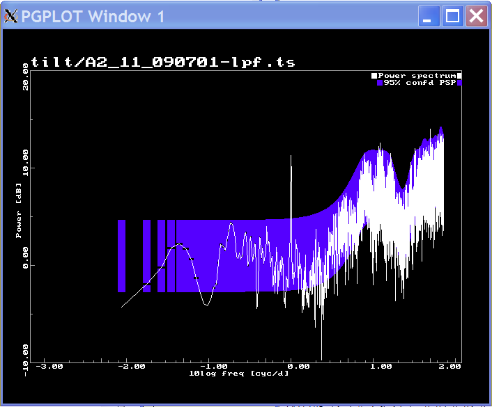
# Finally, a power spectrum
# First, we need to detect and remove "shocks"
#
detect-shocks 0.01 -f tilt/shocks.tse
tilt/A2_11_090701-lpf.ts
#
setenv sasm03_input tilt/A2_11_090701-lpf.ts
setenv sasm03_output tilt/sasm03.psp
#
sasm03 sasm03-tilt.ins
#
# with sasm03-tilt.ins
21 ^ ${sasm03_input}
41 < sasm03.pef
42 B ${sasm03_output}
Q
¶m
lvllen=-1,
qshlvl=.false.
rec_mrs=-99999.9,
dat_mrs=-99999.9
l_section=8192,
logxax=.true.
target='BIN',
fmt='U'
units='[mV]$'
mx_miss=10000,
dff1=-.999d0, ibeg_burg=24, qrfsp=.false.
qrepair=.true.
lpef=21,pef_order=19, lpef_wh=-1, iun_wh=-1, qrpefsp=.false.
pef_show=11,
pef_order_show=20,15,12,9,7,6,5,4,3,2,1
t_window='KAIS',
p_window=2.2
qgra=.true.
cutlvl=1.d-8
scale=1.d3
q_tsf_edit=.true.,
tsf_edit_name='SHOCKS'
iuspout=42
&end
TSF EDIT SHOCKS
CONT 43 R tilt/shocks.tse
END
#
# Result:
The
tilt
controllers went over-range in the surface waave
action after Maule, Feb. 27, 2010. The following recipe
~accomplished a restoration of the signal:
setenv RESIDEDIT -Etilt-unclip.tse,U
daily-resid -x 11,19,12,20
-L TX-PWR,VAL -L TY-PWR,VAL -L TX-BAL,VAL -L TY-BAL,VAL -NT -T
tbxy RAW_o054/A2100227.054
tilt-unclip.tse:
TSF EDIT U
DEL > 9.9
UNCLIP T=1.d-5 I=1000 S=4
O=P+
END
Result:
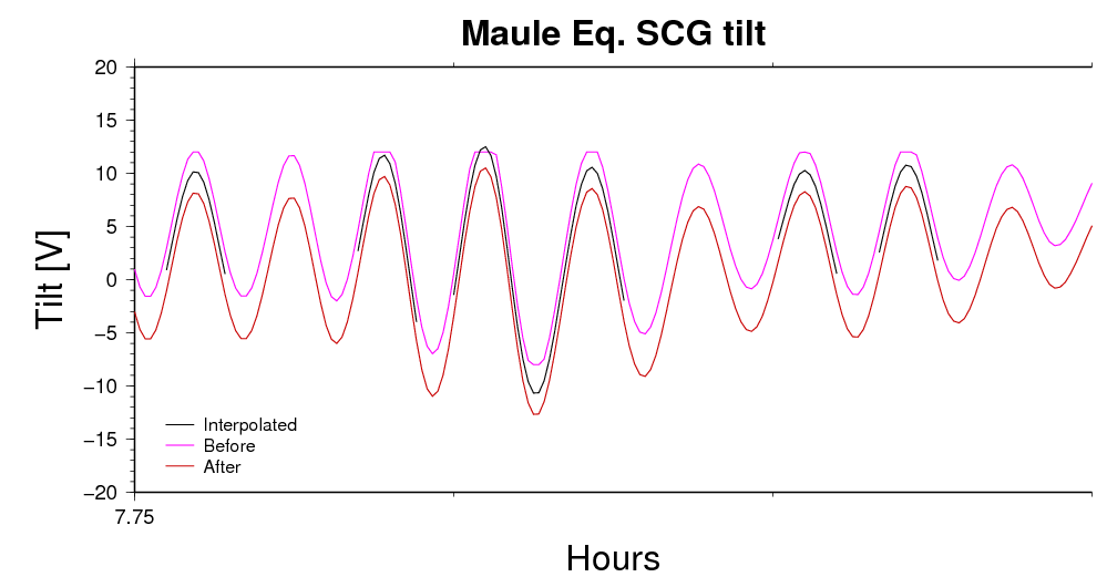
The tick interval on the time axis is 1 minute. The "After" and
the "Interpolated" curves have been moved by -2 and +2 Volt,
respectively.
For more on the subject of unclipping, see "Displacements
from
gravity" and "Signal
Restoration".
For the plot, use the following two lines in tilt-unclip.tse to
prepare output:
OUTTS U=51
< o/Chile-TXPWR-unclip-1s.ts
OUTTS W U=51 <
o/Chile-TXPWR-uncpre-1s.ts
and the plot-init file plot/tilt-unclip.init
Knowing the X- and Y-signals, we would like to obtain the East
and North motion/acceleration or the motion in the direction of
wave propagation and at right-angle. For this purpose
there is a routine that write a tse-file with the appropriate
parameters
~/TD/tiltrot
tiltrot -a 65 -c PWR -o
d/A2_tiq_100227-1s.mc d/A2_tbxy_100227-1s.mc
The 3-component results can be viewed here.
# Si-Diode
thermometers
# We take data from A1 files:
#
tsf2ts-decim -w -W -d 60,0 -r 15,250 -u
13,14 -o therm/ RAW_o054/ A1 0906
# with conversion to K units (Kelvin). The -d 60,0 reduces
the 1-min A1-data sets to 1-hour.
#
# Here is the plot
(ranges manually set, -Y-30 for Neck-T1)
#
# There is a special day found in the output:
#
tslist therm/A1_13_090615-60m.ts -I -qm -C3
| <GetTs->>>
File MRS= -9.99999D+04, test,new= F T
| <GETTS->>>
#21: therm/A1_13_090615-60m.ts N=5992, Skip=0, Miss=0,
Val=5992
| <GETTS->>>
Epoch set: 2009-06-15 - Return t0, dt = 4.0000D+00
[h] 1.0000 [h]
| <main-->>>
after trunc, n,t0= 5992 4.00000000000000
| <Main-->>>
Remove=F DC-value= 3.8660D+01 from column 1
|
<Main-->>>
RMS-dev= 6.8931D+00 from column 1
| <Main-->>>
Min = 3.7471D+01 at 5014 D T
= 2010 01 10 01 00 00 00
| <Main-->>> Max
= 1.6791D+02 at 2094 D T
= 2009 09 10 09 00 00 00
| <Main-->>>
therm/A1_13_090615-60m.ts Total_miss=0, N=5992, Val=5992
#
# so we make another plot around that one day, 2009 09 10,
1-m original sampling.
# In order to exclude that the spike is a unit
conversion problem,
#
tsf2ts-decim -w -W -d 1,0 -r 8,11 -u 13,14
-o therm/ RAW_o054/ A1 0909
#
# again plotting
the result.
Plot
Example: The "human" effect of a group visiting the site and
doing the kneel-down.
cd ~/TD
xchan-units -C
G1-Sig:-776.0 -u -x 5 RAW_o054/A2100414.054 |\
tslist - -A -g'(I4,5I3,f15.0)' -k3 -F1p,e18.10 -C3
-o o/A2_5_100414.ts -I
tslist
o/A2_5_100414.ts -BHc2010,4,14,16 -Un7200 -C3
-Elpf.tse,USBPF -Ff15.5 -I -o o/A2_5_100414-bpf.ts
with lpf.tse
TSF
EDIT USBPF
;
Removes microseisms and tides in 1-s data
FILTER
D:WD
KAIS 100 2.1 0.007 0.07 0.5 0.02
/FILTHR
S 30 20 10 5 1
END
cd ~/TD/plot
setenv
TSPLOT_INIT human.init
t -i TITLE 'Human on
2010-04-14'
t YTITLE "Gravity
[nm/s@+2@+]"
t FILE
../o/A2_5_100414-bpf.ts ../o/A2_5_100414-bpf.ts
etc., creating an init file like
echo Sourcing human.init
set
TSPLOT_PSOUT
= human.ps
setenv
TSPLOT_TITLE
"Human on 2010-04-14"
setenv
TSPLOT_XTITLE
"Hours"
setenv
TSPLOT_YTITLE
"Gravity [nm/s@+2@+]"
set
TSPLOT_FILE
= ( "../o/A2_5_100414-bpf.ts" "../o/A2_5_100414-bpf.ts" )
set
TSPLOT_XAXTYPE
= ( "'-Nf14.7 -n1/3600.'" "Hours" )
set
TSPLOT_TSLIST
= ( "'-D -n1/60.-30 -BHc2010,4,14,16,30'" "'-D -n1/60.-57
-BHc2010,4,14,16,57 -Y10'" )
set
TSPLOT_XAXTYPE
= ( "-Nf14.7" "Minutes" )
set
TSPLOT_LEGTXT
= ( "'Group 1'" "'Group 2'" )
setenv
TSPLOT_XR
"0/30"
setenv
TSPLOT_YR
-20/20
setenv
TSPLOT_YTIX
a10f1
setenv
TSPLOT_XTIX
a10f1
set
TSPLOT_LEGY=3.5
source hans-tsplot.env
ps2png -rr -m -d 144x144 human.ps
If things go wrong, you might need to
unset noglob
Many signals
tsf2ts-decim -w -W -c 1-48 -r
2,2 -d 1,0 -o signals/ RAW_o054/ A1 1002
cd plot
Prepare an init file:
echo Sourcing many-signals.init
set
TSPLOT_FILE = ( )
set
TSPLOT_LEGTXT = ( )
foreach
i ( `fromto $1 $2` )
@ ii =
$i
set
TSPLOT_FILE = ( $TSPLOT_FILE ../signals/A2_${ii}_100203-60s.ts )
set
TSPLOT_LEGTXT = ( $TSPLOT_LEGTXT `xchan-units -H $i
../RAW_o054/A2100203.054` )
end
#
set TSPLOT_XAXTYPE = ( '-Nf8.4 -n/60.' 'Hour' )
setenv TSPLOT_XR "0/24"
setenv TSPLOT_XTIX "a1f0.166666667"
setenv TSPLOT_XTITLE "Hour"
setenv TSPLOT_TITLE "2010-02-03"
set TSPLOT_TSLIST = ( "'-SOM0.5 -Un1440'" "'-SOM0.5 -Un1440
-Y"'$ic'"'" )
setenv TSPLOT_YR "-1/10"
setenv TSPLOT_YTITLE "Signal [mapped]"
set TSPLOT_PSOUT = ( 'many-signals.ps' )
setenv TSPLOT_SIZE "9/6"
setenv TSPLOT_XR "-6/24"
set TSPLOT_LEGSIZ = ( '1.7/5.45' )
set TSPLOT_LEGY = ( 0.4 )
set pen = ( 0/0/200 '`autocolor 15 $i`' )
set pth = ( 3 3 )
source hans-tsplot.env
GGS data
Example:
#
tsf2ts-decim -g -w -r 28 59 -d 1 -o GGS/ RAW_o054/ G1 1002
#
creates a 1-s GGS file for Feb 28
through Mar 31. Option -w generates the header from TD/GGS-header.054
Inside, this step uses special options to tslist worth
documenting:
tslist ... -TGGSJ
upon tsf2ts-decim -g -w ...
(it writes a block-start record
first).
In the daily loop, the option is subsequently changed to -TGGS since
we don't want block starts every midnight.
#
tslist ... -qqq -zo999.99,99.0
is supposed to write missing
records as symbolic values gicen in the -zo option.
If the day range extends over more than 1
day, the output file name will run the date YYMM00
Else the file is considered a daily file, and the date in
the file name is YYMMDD as in
#
foreach day ( `fromto 28 59` )
tsf2ts-decim -g
-w -r $day $day -d 1 -o GGS/ RAW_o054/ G1 1002
end
#
Send to Crossley by
#
ftp ftp.eas.slu.edu
cd pub/incoming/ggp
bin
hash
put ...
#
Free Oscillations
The time-frequency xyz diagram on the www/SCG/ page is produced with
~/TD/daily-fo-pdg
Periodograms:
We have made a succession of files, 3 days 15s in ~/TD/fo/
foreach d ( `fromto 27 87` )
@ e = $d + 3
myfo -o fo -f MYFO -c LOOK
2010 02 $d $e
end
with rmsmode.tse
TSF
EDIT MYFO
FILTER
D:WD KAIS 240 2.0 0.00022 0.0025 -3600. 0.001
END
(we got quite high sidelobes beyond the upper band edge,
unfortunately)
Make a periodogram:
set f=`calc -f
%16.14f '0.03333333333/10.080'`
foreach file (
fo/fo100[3-4]*.ts )
set o=`echo $file | sed
's/ts$/pdg/'`
tslist $file -Epdgram.tse,PDG
-Nf11.7 -n'*'$f -Ff10.4 -qqq -w $o
end
pdgram.tse:
TSF
EDIT PDG
FILTER
0 1 ' '
1.0
-1.0
REMDC
PERIODOGRAM
U,/NdB To #20159
END
truncation for a faster FFT
The periodograms can be put together to create a 3-d spectrum.
awk '( $1 == "0.0000000" ){
c++ }; {print c,$1,$2}' fo/fo100[3-4]*.pdg | xyz2grd
-Gfo/fo.pdg.grd -I1/0.0033069 -R1/59/0/33.3333333
cd plot
makecpt -Cseis -T-20/40/3 -I
> ! pdg.cpt
grdview ../fo/fo.pdg.grd
-Cpdg.cpt -JX5/5 -R1/59/0.5/1.0 -Ba5f1:d:/a0.1f0.01:mHz:WESN -Qs
> ! fo.pdg.ps
We only plot a narrow frequency band. Notice the 0S0
mode at 0.817 mHz !
Easy preparation of 1-min data for a
strech of days
In May 2013 we had a cron job running:
00 08 * * * /home/hgs/TD/daily-fo-pdg.sh -e Kamchatka -A >
/home/hgs/TD/logs/daily-fo-pdg.log 2>&1
Example for the Sendai earthquake
foreach d ( `fromto 0 7` )
set ymd=`YMD 110311 $d`
tslapp -n 1 -L 'G|R'
d/G1_gar_${ymd}-1s.mc -Edeci.tse,60 -C3 -qbe -Un1440 -o
d/G1_r_${ymd}-60s.ts
end
set ymd=`YMD 110311 8`
tslapp -n 0 -L 'G|R'
d/G1_gar_${ymd}-1s.mc -Edeci.tse,60 -C3 -qbe -Un1440 -o
d/G1_r_${ymd}-60s.ts
tslapp -n 8
d/G1_r_110311-60s.ts -I -C3 -qbe -o d/G1_r_110311-19-60s.ts
tsl d/G1_r_110311-19-60s.ts -Epdgram.tse,PDG
-n'*1.356336805555556E-3' \
-N -qqq -Ff12.5 -w o/G1_r_110311-19-60s.pdg
~/bin/YMD is a recent script; central code fragment:
JDC -f3i2.2 -A$2 -y2k
-F'(3i2),6' -D $1
foreach d ( `fromto 0 7` )
set ymd=`YMD 110311 $d`
tslapp -n 1 -L 'G|R'
d/G1_gar_${ymd}-1s.mc -Ermsmode.tse,MYFO15 -C3 -qbe -Un5760 -o
d/G1_r_${ymd}-15s.ts
end
set ymd=`YMD 110311 8`
tslapp -n 0 -L 'G|R'
d/G1_gar_${ymd}-1s.mc -Ermsmode.tse,MYFO15 -C3 -qbe -Un5760 -o
d/G1_r_${ymd}-15s.ts
tslapp -n 8
d/G1_r_110311-15s.ts -I -C3 -qbe -o d/G1_r_110311-19-15s.ts
tsl d/G1_r_110311-19-60s.ts -Epdgram.tse,PDG
-n'*1.356336805555556E-3' \
-N -qqq -Ff12.5 -w o/G1_r_110311-19-15s.pdg
Here is the source script sendai-fo-60s-pdg.env
It prepares a low-frequency section of a periodogram of the first
three days, starting 740 samples after midnight 2011-03-11
adds the FO-symbols ot the REM collection (Seism/FO/Laske). I put it
here since forthcoming updates might specialise it even further.
No call-line parameters.
set
begin=110311
if (
! -r o/G1_r_${begin}-4d-60s.ts ) then
foreach
d
(
`fromto
0
7` )
set
ymd=`YMD ${begin} $d`
tslapp
-n 1 -L 'G|R' d/G1_gar_${ymd}-1s.mc -Edeci.tse,60 -C3 -qbe -Un1440
-o d/G1_r_${ymd}-60s.ts
end
#set
ymd=`YMD ${begin} 8`
#tslapp
-n
0 -L 'G|R' d/G1_gar_${ymd}-1s.mc -Edeci.tse,60 -C3 -qbe -Un1440 -o
d/G1_r_${ymd}-60s.ts
tslapp
-n 4 d/G1_r_${begin}-60s.ts -I -C3 -qbe -o
o/G1_r_${begin}-4d-60s.ts
endif
setenv
PDGDB
setenv
PDGFROM
740
setenv
PDGDUR
4320
set
df=`tslist o/G1_r_${begin}-4d-60s.ts -Epdgram.tse,VPDG -n1 -N -qqq
-Ff12.5 -I | awk '/Spectrum: FNy/{printf "%12.10f\n", 1000*$7}'`
tsl
o/G1_r_${begin}-4d-60s.ts -Epdgram.tse,VPDG -n'*'$df \
-N
-qqq
-Ff12.5
-w
o/G1_r_${begin}-3d-60s.pdg
echo
df=$df
cd
plot
psxy
../o/G1_r_${begin}-3d-60s.pdg -R0.2/1/0/2 -JX10/4 -K \
-Ba0.1f0.01:"Freq. [mHz]":/a1f0.1:Pwr:WeSn -W3/0 \
> ! sendai-fo-3d.ps
rem-modes
-a
1.2
-s
0.05
-l |\
psxy
-R
-JX
-O
-K -Sc0.1 -G0 -W1/0 >> sendai-fo-3d.ps
rem-modes
-T
-a
1.2
-s
0.0 -l |\
psxy
-R
-JX
-O
-K -Sc0.1 -G0/0/255 -W1/0/0/255 >> sendai-fo-3d.ps
rem-modes
-a
1.5
-s
0.1
|\
pstext
-R
-JX
-O
-K >> sendai-fo-3d.ps
rem-modes
-T
-a
1.5
-s
0.1 |\
pstext
-R
-JX
-O
-G0/0/255 >> sendai-fo-3d.ps
(
setenv PS2PNG_OPT '-crop 1684x794+0+391 ' ; ps2png -m -rr -d
144x144 sendai-fo-3d.ps )
convert
-resize
50% PNG/sendai-fo-3d.png PNG/sendai-fo-3d-small.png
cd
..
echo
ready plot/sendai-fo-3d.ps
Daily
residuals, micro-seismic spectrum, shocks, and cleaned low-rate
data
Daily RMS time series and statistics
daily-rms -rc
rms/minmax-rms.dat -wca rms/rms-all.tsf -o rms/rms-all.ts -d 1H
d/G1_gar_*-1s.mc
daily-rms -rc
rms/minmax-rms.dat -wca rms/rms-all.tsf -o rms/rms-all.ts -L 'G|B'
-d 1H d/G1_garb_*-1s.mc
produces the following files:
rms/minmax-rms.dat
rms/rms-all.tsf
rms/rms-all.ts
and intermediate file rmstst.ts
daily-rms
contains a few useful TSF
EDIT sections. The command above runs TSF
EDIT 1HRMS as -d 1H is appended
with RMS
by default.
A section TSF EDIT 1HRMS produces
1-hour RMS in the following way
x(j) -> Narrow-Band-Filter
-> x(j)**2 -> y = median(length 1h, move 1h) -> sqrt(y)
-> x(k)
j=1,n,3600; k=1,n/3600
TSF EDIT 1HRMS
FILTER D:WD KAIS 32 2.0 0.1 0.5 1.0 0.25
X**2
MEDIANFI 3600 M=3600 To #90001
SQRT
TRUNC N=24
END
A now obsolete section TSF
EDIT
1HRMSOLD produces 1-hour RMS-samples with a
2-hour raised-cosine window.
To invoke other files for editing, use option -E
file,target
and don't specify -d
-E daily-rms,1HRMSOLD
for the deprecated version e.g.
In daily-rms,
besides 60RMS 600RMS and
1HRMS there is a
section 1HMAX
that
produces 1H abs-max values
daily-rms -rc rms/minmax-max.dat -wca rms/max-all.tsf -o
rms/max-all.ts -E daily-rms,1HMAX d/G1_gar_*-1s.mc
Here is daily-rms section 60RMS
TSF
EDIT 60RMS
FILTER 0 1
' '
1.0 -1.0
MOVRMS 60
120 I=59 M=W To #86780
; To
#86400 + INITIALMOVE + HALFLENGTH
TRUNC
N=1440
MEDIAN
END
Explanation
MOVRMS
We use
the raised-cosine window version (M=W), length 2 * 120 +1,
go in steps of 60 samples
TRUNC N=1440 Output a full
day (86400/60 = 1440)
MEDIAN
provides a report of min, max, and median of
the time series, which is now the sliding-RMS.
FILTER 0 1 ' '
1.0 -1.0 We
do filtering = differencing to get rid of noise colour and tides and
other slow things.
Daily Power spectrum and 3d colour
plot
run-daily-psp-vs-time -px -F
o/collect_sp_1006 2010 06 01 2010 06 30
retrieves d/G1_gar_${yymmdd}-1s.mc files by default, execs daily-psp
and does the plotting.
A daily signature?
setenv APPENDFILE
`nextfile d/G1_gar_100331-1s.mc`
setenv APPENDLABEL 'G|R'
tslist
d/G1_gar_100331-1s.mc -L'G|R' -C3 -Hc2 -soh-2 -Eappend.tse,L
-Eeditshocks.tse,SD60 -F1p,e12.4 -Un1440 -I -D -o tmp.ts
cleans for shocks, decimates to 1-min and changes time to zone time
UT +2h
Here's how to find the days when the clock is
adjusted for summer time:
daylight
2008 2009 2010 2011
2008 On: 54555.0 Off:
54765.0
2009 On: 54919.0 Off:
55129.0
2010 On: 55283.0 Off:
55500.0
2011 On: 55647.0 Off:
55864.0
Here's how to find the hour shift w.r.t. UTC:
is_daylight
20100623
2
or even
set dh = `is_daylight d/G1_gar_100623-1s.mc`
and use $dh in
setenv APPENDFILE `nextfile
d/G1_gar_100623-1s.mc`
tslist
d/G1_gar_100623-1s.mc -L'G|R' -C3 -Hc$dh -soh-$dh
-Eappend.tse,L -Eeditshocks.tse,SD60 -F1p,e12.4 -Un1440 -I -D -o
tmp.ts
List all files associated with weekdays, no holidays:
is_kod -H 12345 d/G1_gar_??????-1s.mc
... collect, now also removing the holiday seasons
is_kod -H 12345
d/G1_gar_??0[1-6]??-1s.mc d/G1_gar_??0[8-9]??-1s.mc
d/G1_gar_??1???-1s.mc | sort > working-day.lst
... collect the labour-free days:
is_kod +H 06 d/G1_gar_??????-1s.mc > tmp.lst
ls d/G1_gar_??07??-1s.mc >> tmp.lst
sort tmp.lst >
lazy-day.lst
...and manually delete 100227 100228 avoiding the Maule
earthquake
Then we can run a script like
set daytype=working # alt. set daytype=lazy
source daily-signature
where daily-signature runs
rm -f ${daytype}-day.stack
foreach file ( `cat
${daytype}-day.lst` )
setenv APPENDFILE
`nextfile $file`
setenv APPENDLABEL
'G|R'
set dh =
`is_daylight $file`
tslist $file -L'G|R'
-C3 -Hc$dh -soh-$dh -Eappend.tse,L -Eeditshocks.tse,SD60
-F1p,e12.4 -Un1440 -I -D -o tmp.ts
accustack tmp.ts
${daytype}-day.stack
# accustack -c
o/${daytype}-day-c.ts tmp.ts ${daytype}-day.stack
end
accustack -s
${daytype}-day.stack o/${daytype}-day.ts
The out-commented line avoids accumulating data that "differs too
much" from a previously established average signature (default
threshold 20 nm/s^2)
Diagnostic plot
We want to inspect a few channels in A2 files over a short period of
time, generally at the 1s sampling interval.
Program to use: hms-plot
cd ~/TD
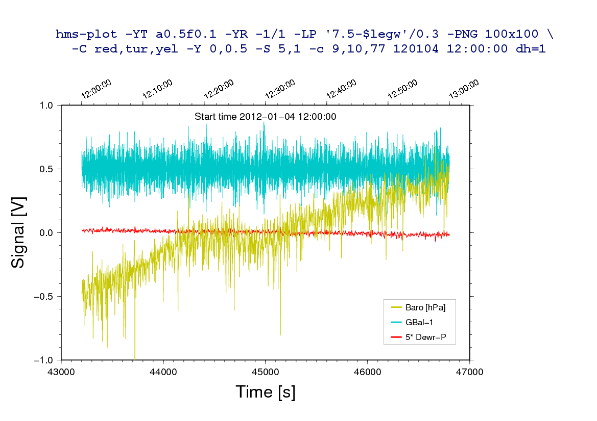
hms-plot
-YT a0.5f0.1 -YR -1/1 -L '7.5-$legw'/0.3 -PNG 100x100 -C
red,tur,yel \
-Y 0,0.5 -S 5,1
-c 9,10,77 120104 12:00:00 dh=1
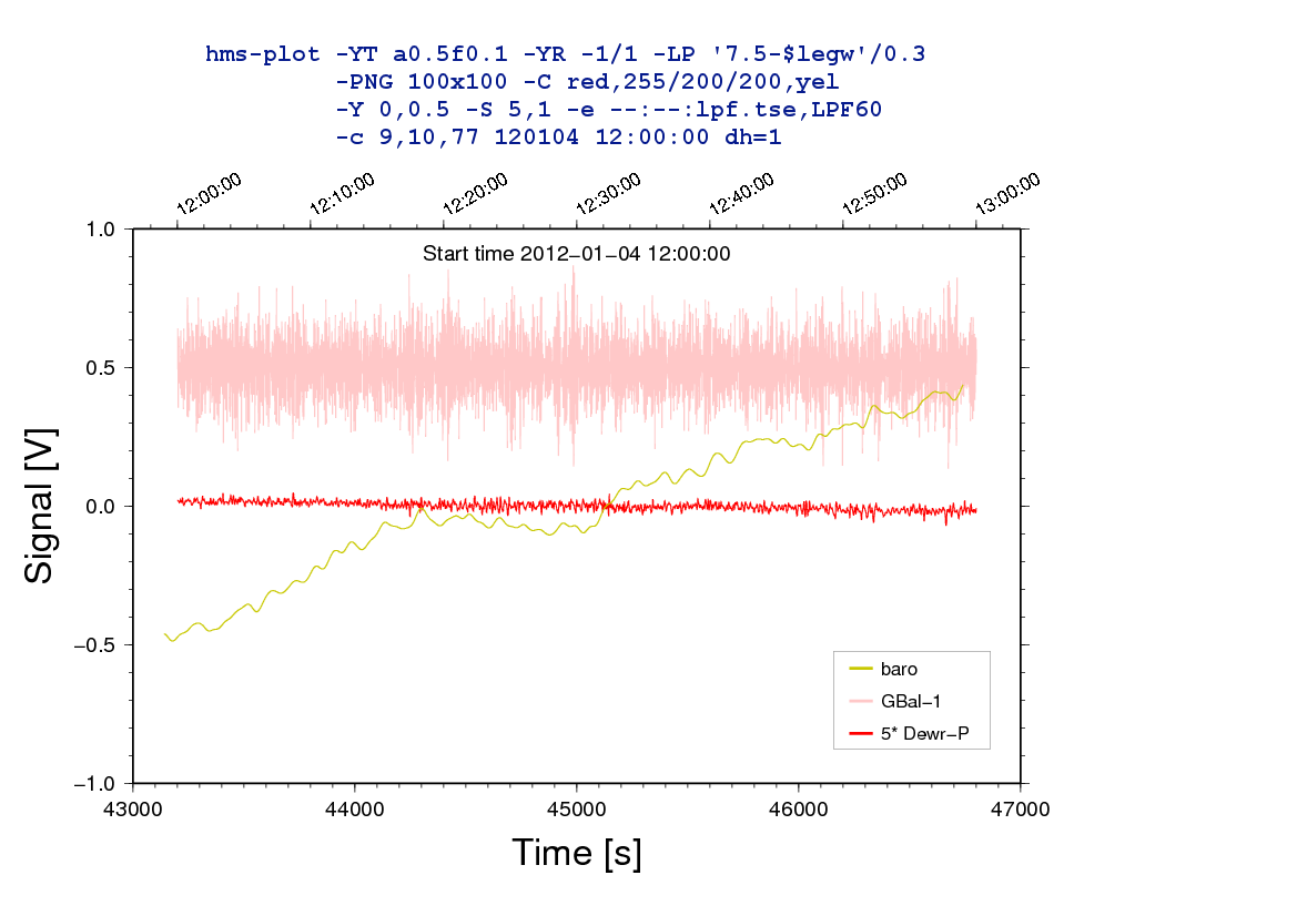
hms-plot
-YT a0.5f0.1 -YR -1/1 -LP '7.5-$legw'/0.3 -PNG 100x100 \
-C
red,255/200/200,yel -Y 0,0.5 -S 5,1 -e --:--:lpf.tse,LPF60 -c
9,10,77 120104 12:00:00 dh=1
Sequence
of
periodograms and a 2-d histogram
Procedures:
~/TD/:
pdgram.tmp.prc pdgram.tse
~/TD/plot/: tmp.prc
rastered-pdg.env
.bye