News from GWR 054, the Superconducting Gravimeter at Onsala Space Observatory

2013 May 25

GGP-DATA
Live page and much more | Free Oscillations  |  Displacements from GravityFun stuff   |  Stormy weather  |  Kattegat loading  |
Does the 20m radio telescope cause disturbances?  |  Noise  |  Earthquakes | Hum

Visit GWR Instruments - the manufacturer of the gravimeter.

Recent news


Free oscillations time-frequency periodograms
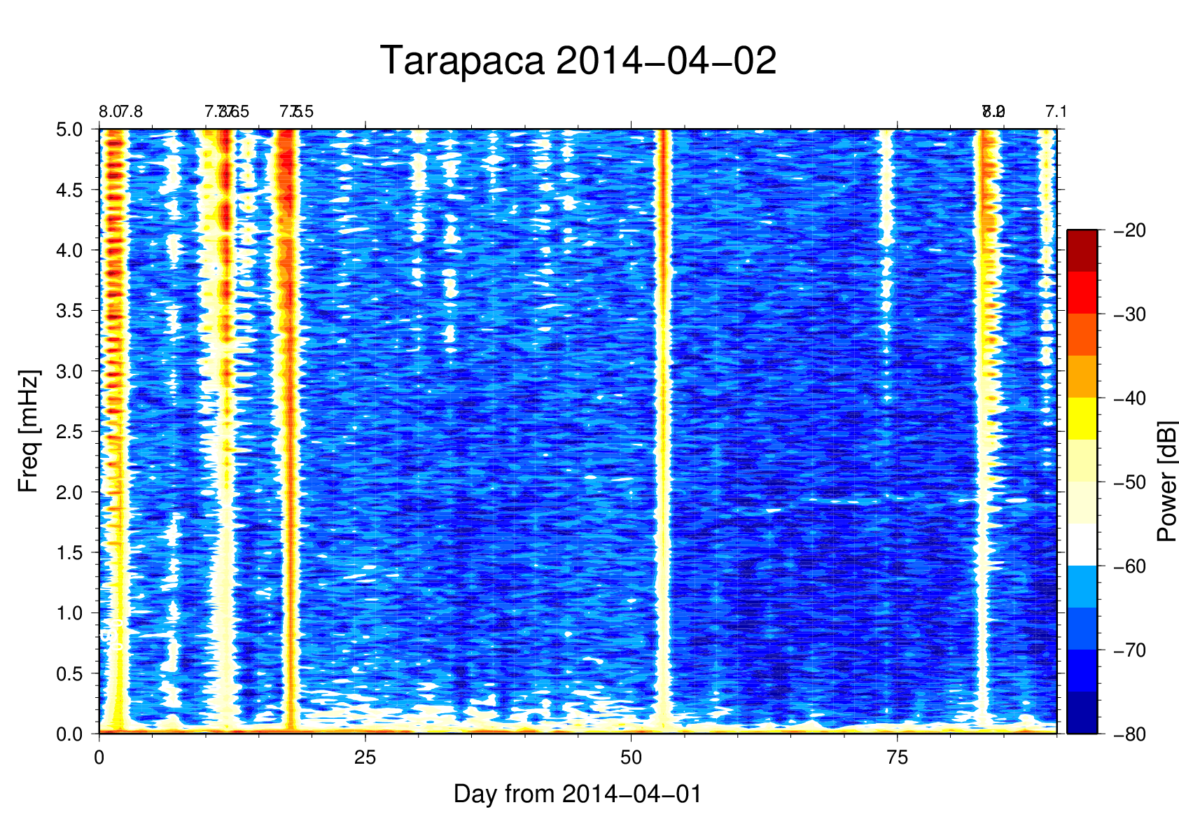
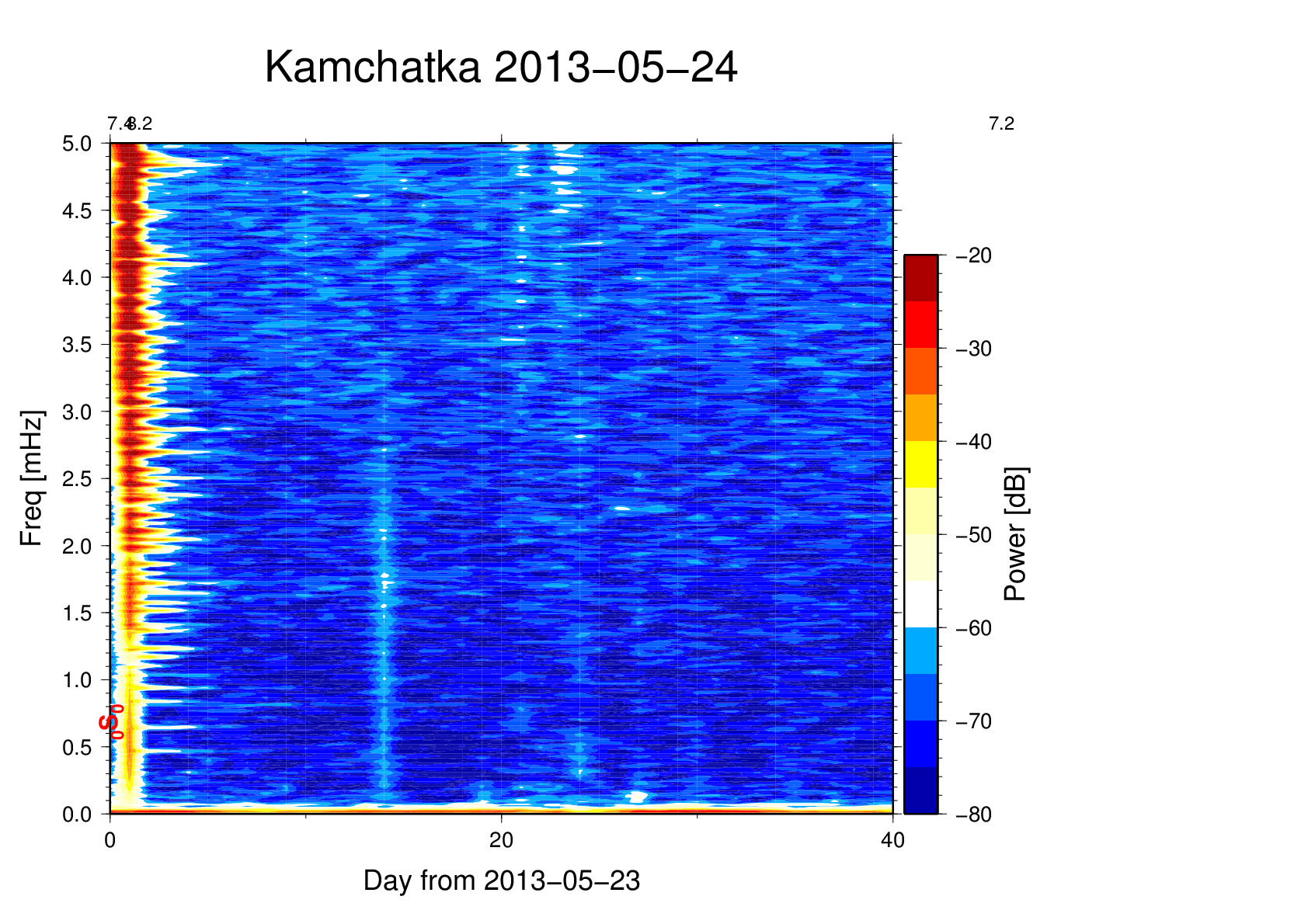
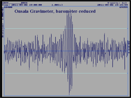
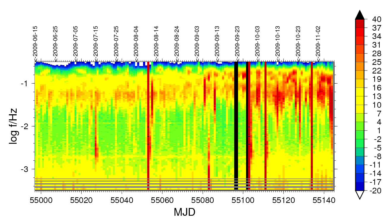
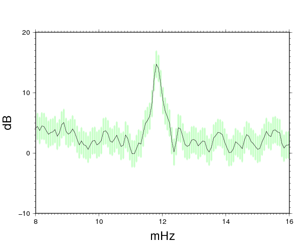
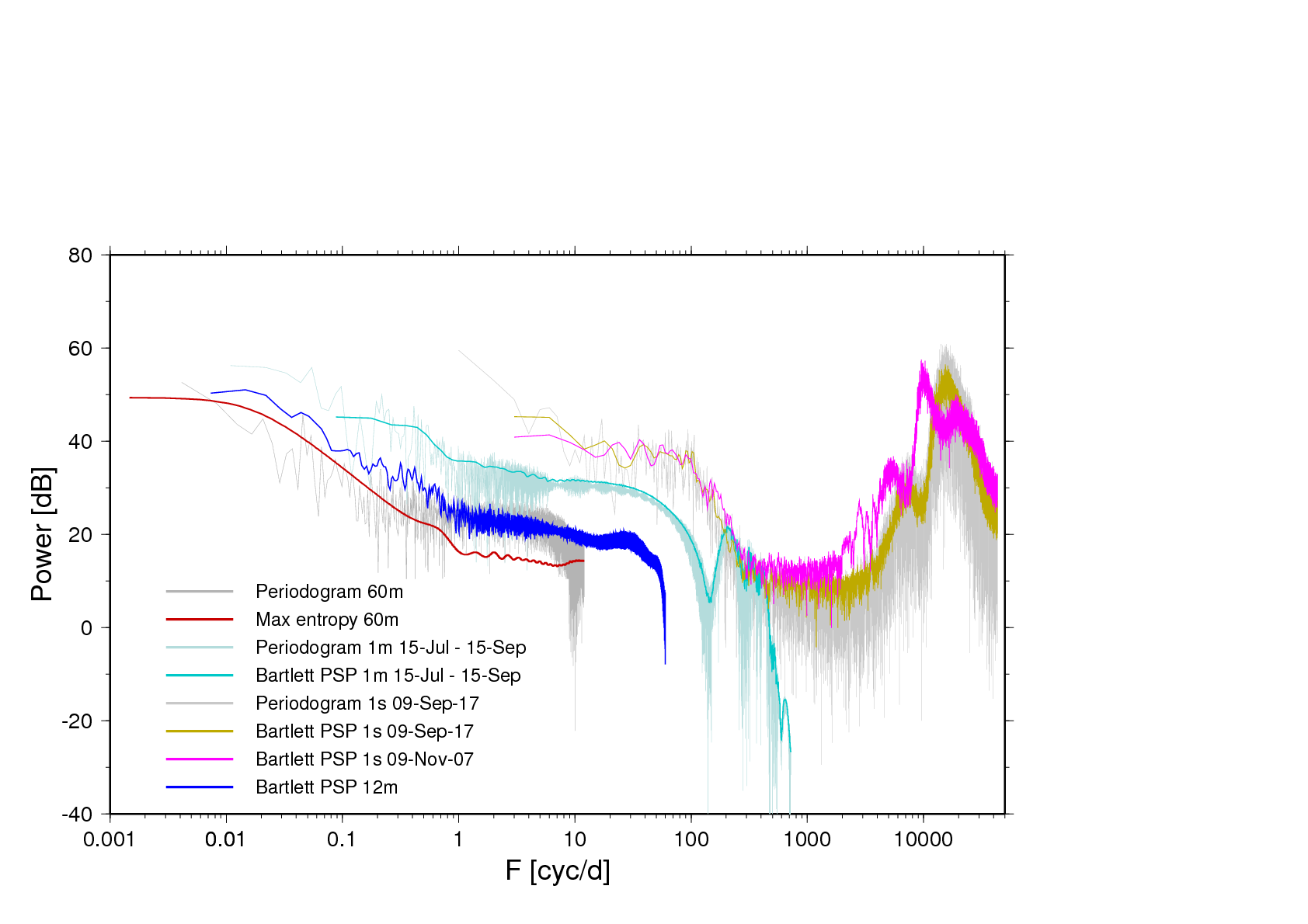
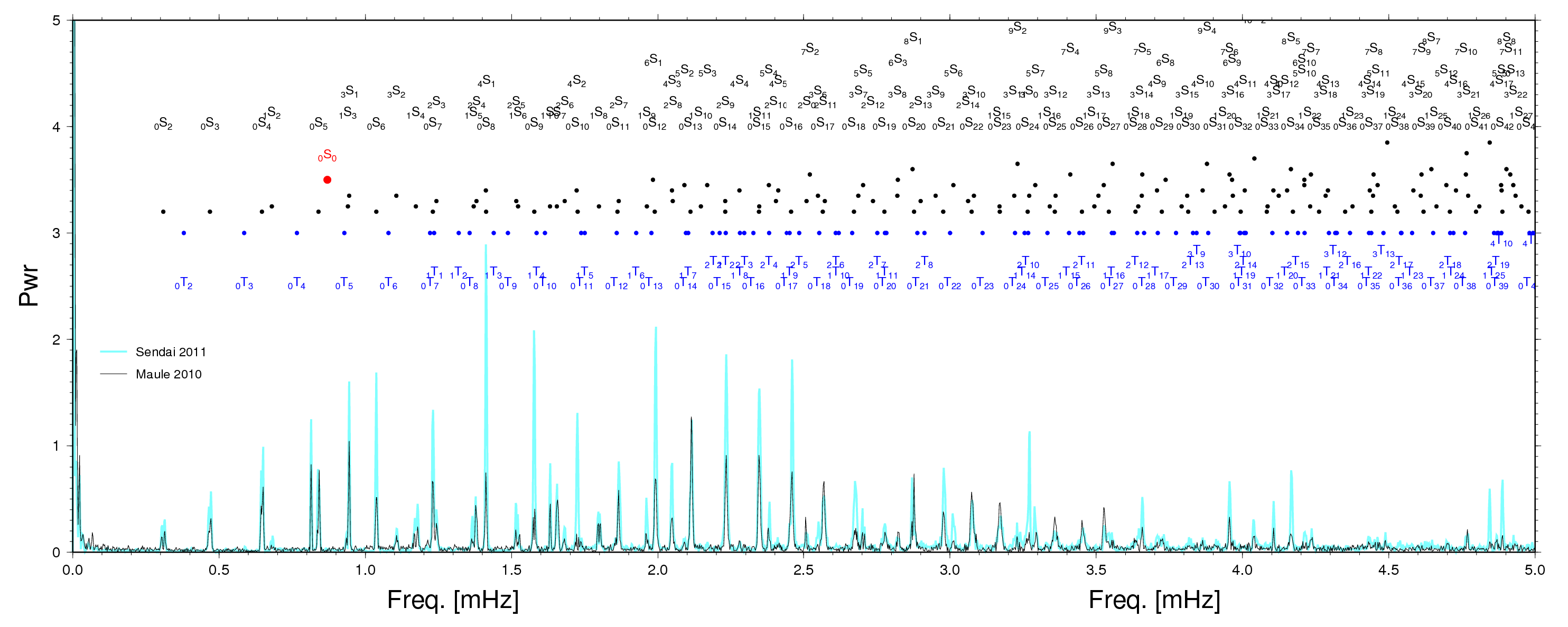
Automatically updated every morning 8 a.m. (click on image to show full size). Temporal resolution is one day. Estimated from 15-s data, thus frequency resolution is 0.011574 mHz. Although this resolution is not optimum for detection of the 0S0-mode (0.81699 mHz), the use of a Hanning window warrants enough amplitude response to make the signal visible.
A long-time series' periodogram, five days of 30-s data. The earthquake has not excited the "balloon" mode 0S0 to any efficient degree. The signal strength is 100 times less compared to Tohoku 2011-03-12, cf. below.


A smack of the Chelyabinsk meteorite whack on February 15, 2013 ? It hit the ground 03:20 UT.


(Click on image to show full size). The figure shows how two instruments at OSO recorded the seismic waves caused
by the meteoritic shock, the gravimeter (SCG) and the seismometer (operated by Uppsala university as a station in their
SNSN network). The features at minutes 36-39 are the surface waves from the shock as they pass through Onsala. 
The small wiggles earlier, at minute 23, are probably identified as the body wave P. The wave form starting around 
minute 70 looks like an earthquake unrelated with the meteorite; Tonga, 03:02 M=5.8, is a candidate (thanks, Michel van Camp!),
however, the text above needs reassessment. The alleged meteorite shock might have been mixed up with
an early phase of the Tonga earthquake (PKP) . 


The earthquake of 2012-Jan-08 17:14 UT near Falkenberg - see Earthquakes page.


The earthquake west of Halmstad, 2012-AUG-06


Uuups, what was that?!
 
(Earthquakes in Central/Western Europe)


Free oscillations from Maule (2010) and Sendai (2011) in comparison
(click for larger image)        
from four days of 60s band-pass filtered gravity residuals, 2010-02-28-- and 2011-03-12--, respectively.
The decay of Free oscillations over time   
(click for larger image)    
after Sendai main shock 2011-03-11 05:46 UT


Link to a wide version, 0 to 5 mHz


The 2011-03-11 UT 05:46 Tohoku Mw9.0 earthquake near Sendai, Japan

From 72h Superconducting gravimetry, 1-s data, at Onsala Space Observatory
Appearance of  0T3, a toroidal oscillation, is due to earth rotation, more specifically Coriolis acceleration.
On a non-rotating earthm a toroidal mode would only have horizontal motion. The Coriolos effect
induces a small fraction of acceleration into the vertical, where the gravimeter can sense it.

The annotation of the 0S0 mode is misplaced in this plot, should be at 0.817 mHz, sorry!

For more information, go to our page on Free Oscillations

Hans-Georg Scherneck, March 17, 2011


Figure 1 - 1-min data since the beginning of the superconducting gravimeter operations at 13 June 2009 until 22 February 2010. Fitting an empirical tidal model produces the blue curve as a residual. The tide model includes the effect of Polar Motion. Fitting the barometer recording with an empirical coefficient produces the purple curve as a residual. 


Figure 2 - The tides+baro residual from Figure 1 is repeated here. We fit a simple drift model (blue curve) consisting of an exponential and a straight line.
The exponential has a start value of -372 nm/s  and a relaxation constant (1/e-time) of 1,220 h (about 51 days).  The linear drift is 0.74 nm/s per day.


Figure 3 - Subtracting the drift curve (and nothing else) from the tide+baro residual of the previous figure retains those difficult-to-model variations of gravity (blue curve). We can mention two obvious sources: Atmospheric density structures that cause gravity variations that cannot be represented by a simple stationary one-coefficient proportionality with surface pressure variation. And water level variations in near-by Kattegat (purple line covering October and November 2009). These effects will be subject to future investigations when we have a continuous record of the Ringhals tide gauge. For the time being we note that the peak-to-peak variation is on the order of the specified accuracy of Absolute Gravimeter FG5. And perhaps twice the repeatability that can be achieved with individual FG5's.
   The black line shows a sliding-RMS, a kind of VU-metre like on your stereo equipment at home. Many of the peaks appear to correlate with major teleseismic events (red circles) obtained from http://earthquake.usgs.gov/earthquakes/ . The smallest circles reperesent Mw 6.5 events.


Figure 4 - Daily Power spectra, exhibiting the varying level of microseismic background noise (orange and red zones above 0.05 Hz). The vertical red strokes are the effect of earthquakes. The black strokes occur at dates when earthquakes have been too strong; they had caused the sensor to hit the range stops. Just above 0.01 Hz a thin line with elevated signal level at constant frequency is visible, a high-quality resonance. This is the eigenfrequency of the superconducting sphere swaying in the shallow magnetic valley that provides the restoring force of the sensor.


Figure 4.a - The eigenfrequency of the superconducting sphere (correspoding period is 84.7 s)

 
Fig. 5  - Power spectra of various time scales, from individual days to 8.5 months. In the microseismic domain, 8000 cycles per day or above, two days are shown that differed with respect to storm activity in the North Atlantic. The brownish curve is from a more quiet day, the pink one from a stormy day causing high waves on the European shelves. The hanging high-frequency ends are effects of decimation filters. The Bartlett power spectra use a spectral domain with 8192 spectral bins and a Kaiser-Bessel window on the autocovariance with a truncation point of 1/2 of this number. The Maximum entropy spectrum is based on a prediction error filter of length 40. The capping of the noise poower towards lower frequencies is probably not significant - the finite filter length makes this behaviour inevitable.  

Hans-Georg Scherneck